What does it mean when an election forecaster tells us that a candidate has a 90% chance of winning? In classical (frequentist) statistics, probability refers to long-run frequencies of events. A parameter like the true proportion of voters supporting a candidate is a fixed but unknown number—it doesn’t make sense to assign it a probability.
Bayesian statistics takes a different view: probability represents our degree of belief about uncertain quantities. Under this framework, we can legitimately say “there is a 90% probability that candidate A will win” because we’re expressing our uncertainty about the outcome.
This chapter introduces Bayesian thinking and shows how it provides a principled framework for combining prior knowledge with observed data.
40.2 Bayes’ Theorem: The Foundation
Bayes’ theorem relates conditional probabilities:
\[
P(A \mid B) = \frac{P(B \mid A) \cdot P(A)}{P(B)}
\]
This simple equation has profound implications. It tells us how to update our beliefs about \(A\) after observing evidence \(B\).
A Diagnostic Test Example
Consider a test for cystic fibrosis with 99% accuracy:
Despite the test having 99% accuracy, the probability of having the disease given a positive test is only about 2.4%. This counterintuitive result arises because the disease is so rare—most positive tests are false positives from the large healthy population.
# Probability of disease given positive testcat("\nP(Disease | Positive test):",round(sum(test =="+"& outcome =="Disease") /sum(test =="+"), 3), "\n")
P(Disease | Positive test): 0.027
The simulation confirms our calculation: despite the high test accuracy, most people who test positive are actually healthy because the disease is so rare.
The Base Rate Fallacy
Ignoring the base rate (prior probability) of a condition leads to dramatically wrong conclusions. This is critical in medical testing, forensic evidence, and any diagnostic situation. Always consider:
How accurate is the test? (sensitivity, specificity)
How common is the condition? (base rate/prevalence)
What population is being tested? (targeted vs. general screening)
40.3 From Bayes’ Theorem to Bayesian Inference
Bayes’ theorem becomes a framework for statistical inference when we apply it to unknown parameters:
The posterior combines what we knew before (prior) with what the data tell us (likelihood).
40.4 Hierarchical Models: Shrinkage and Borrowing Strength
One of Bayesian statistics’ most powerful applications is hierarchical modeling, where we model variability at multiple levels. This allows us to “borrow strength” across related observations.
A Baseball Example
Consider José Iglesias, a baseball player who in April 2013 had the following statistics:
Month
At Bats
Hits
AVG
April
20
9
.450
A batting average (AVG) of .450 is extraordinarily high—no player has finished a season above .400 since Ted Williams in 1941. How should we predict José’s season-ending average?
The frequentist approach uses only José’s data. With \(p = 0.450\) as our estimate and \(n = 20\) at bats:
A 95% confidence interval is \(.450 \pm 0.222\), or roughly \(.228\) to \(.672\). This interval is wide and centered at .450, implying our best guess is that José will break Ted Williams’ record.
The Bayesian approach incorporates what we know about baseball players in general.
The Prior: What Do We Know About Batting Averages?
Let’s examine batting averages for players with substantial at-bats over recent seasons:
Code
library(Lahman)
Error in `library()`:
! there is no package called 'Lahman'
batting_data |>ggplot(aes(AVG)) +geom_histogram(bins =30, fill ="steelblue", color ="white") +facet_wrap(~yearID) +labs(x ="Batting Average", y ="Count",title ="MLB Batting Averages by Year")
cat("SD of batting averages:", round(sd(batting_data$AVG), 3), "\n")
Error:
! object 'batting_data' not found
The average player has an AVG around .275 with a standard deviation of about 0.027. José’s .450 is over six standard deviations above the mean—an extreme anomaly if taken at face value.
The Hierarchical Model
We model the data at two levels:
Level 1 (Prior): Each player has a “true” batting ability \(p\) drawn from a population distribution: \[
p \sim N(\mu, \tau^2)
\]
Level 2 (Likelihood): Given ability \(p\), observed performance \(Y\) varies due to luck: \[
Y \mid p \sim N(p, \sigma^2)
\]
From the data: - Population mean: \(\mu = 0.275\) - Population SD: \(\tau = 0.027\) - Individual sampling error: \(\sigma = \sqrt{p(1-p)/n} \approx 0.111\)
The Posterior: Combining Prior and Data
For this model, the posterior distribution has a beautiful closed form. The posterior mean is:
\[
E(p \mid Y = y) = B \cdot \mu + (1-B) \cdot y
\]
where the shrinkage factor\(B\) is:
\[
B = \frac{\sigma^2}{\sigma^2 + \tau^2}
\]
This is a weighted average of the population mean \(\mu\) and observed data \(y\). The weights depend on: - How much individual variation there is (\(\sigma\)) - How much population variation there is (\(\tau\))
When individual uncertainty is high relative to population variation, we “shrink” more toward the population mean.
The Bayesian estimate “shrinks” José’s .450 toward the population average, giving a predicted true ability of about .285. The 95% credible interval is much narrower than the frequentist interval.
The Outcome
Here’s how José actually performed through the season:
Month
At Bats
Hits
AVG
April
20
9
.450
May
26
11
.423
June
86
34
.395
July
83
17
.205
August
85
25
.294
September
50
10
.200
Total (w/o April)
330
97
.294
His final average (excluding April) was .294—almost exactly what the Bayesian model predicted! The hierarchical approach correctly recognized that his early performance was partially luck and regressed his prediction toward the population mean.
Code
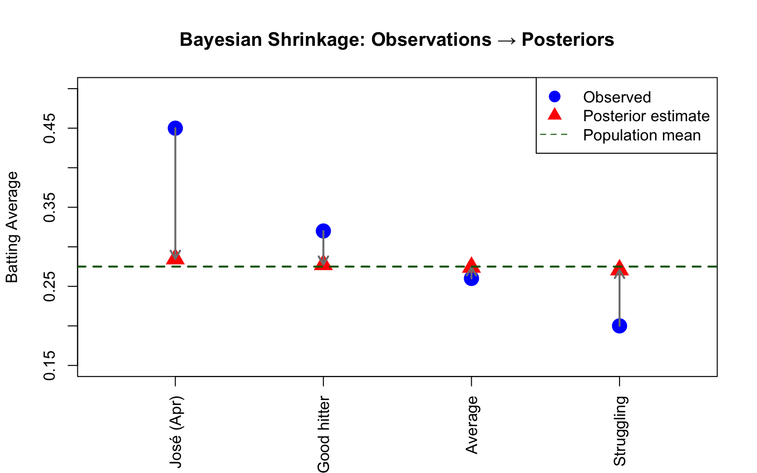
# Visualize shrinkageobservations <-c(0.450, 0.320, 0.260, 0.200)labels <-c("José (Apr)", "Good hitter", "Average", "Struggling")# Calculate posteriors for eachposteriors <- B * mu + (1- B) * observations# Plotplot(1:4, observations, pch =19, cex =2, col ="blue",ylim =c(0.15, 0.50), xlim =c(0.5, 4.5),xaxt ="n", xlab ="", ylab ="Batting Average",main ="Bayesian Shrinkage: Observations → Posteriors")axis(1, at =1:4, labels = labels, las =2)points(1:4, posteriors, pch =17, cex =2, col ="red")arrows(1:4, observations, 1:4, posteriors,length =0.1, col ="gray50", lwd =2)abline(h = mu, lty =2, col ="darkgreen", lwd =2)legend("topright",c("Observed", "Posterior estimate", "Population mean"),pch =c(19, 17, NA), lty =c(NA, NA, 2),col =c("blue", "red", "darkgreen"), pt.cex =1.5)
Figure 40.1: Bayesian shrinkage pulls extreme observations toward the population mean
Notice how the shrinkage is proportional to how extreme the observation is. José’s .450 shrinks dramatically, while the average player’s .260 barely moves.
40.5 Credible Intervals vs. Confidence Intervals
Bayesian inference produces credible intervals rather than confidence intervals. The interpretation differs:
Frequentist Confidence Interval
Bayesian Credible Interval
Statement
“95% of intervals from repeated sampling would contain the true value”
“There is a 95% probability the true value lies in this interval”
Parameter
Fixed but unknown
Random variable with a distribution
Interpretation
About the procedure
About the parameter
The Bayesian interpretation is often more intuitive: we can directly say “there’s a 95% probability the true batting average is between .233 and .337.”
40.6 Choosing Priors
The prior distribution encodes what we believe before seeing data. Prior choice is both a strength (incorporating domain knowledge) and a criticism (subjectivity) of Bayesian methods.
Types of Priors
Priors fall along a spectrum of informativeness. Informative priors incorporate substantial prior knowledge—for example, a prior for batting average based on historical data might be N(0.275, 0.027²), reflecting that most players hit between .220 and .330. Weakly informative priors provide gentle regularization without imposing strong beliefs; a prior of N(0, 10²) for a regression coefficient allows a wide range of values while preferring smaller effects over extremely large ones. Finally, non-informative or diffuse priors attempt to “let the data speak” by imposing minimal prior constraints—for instance, a uniform prior on [0, 1] for a probability parameter, or an improper prior where P(θ) ∝ 1 across the entire real line.
Empirical Bayes
When we estimate prior parameters from data (as we did with batting averages), this is called empirical Bayes. It’s a practical compromise: we use the data twice—once to set the prior, once for inference—but it often works well in practice.
Prior Sensitivity
It’s good practice to check whether conclusions depend strongly on prior choice:
Code
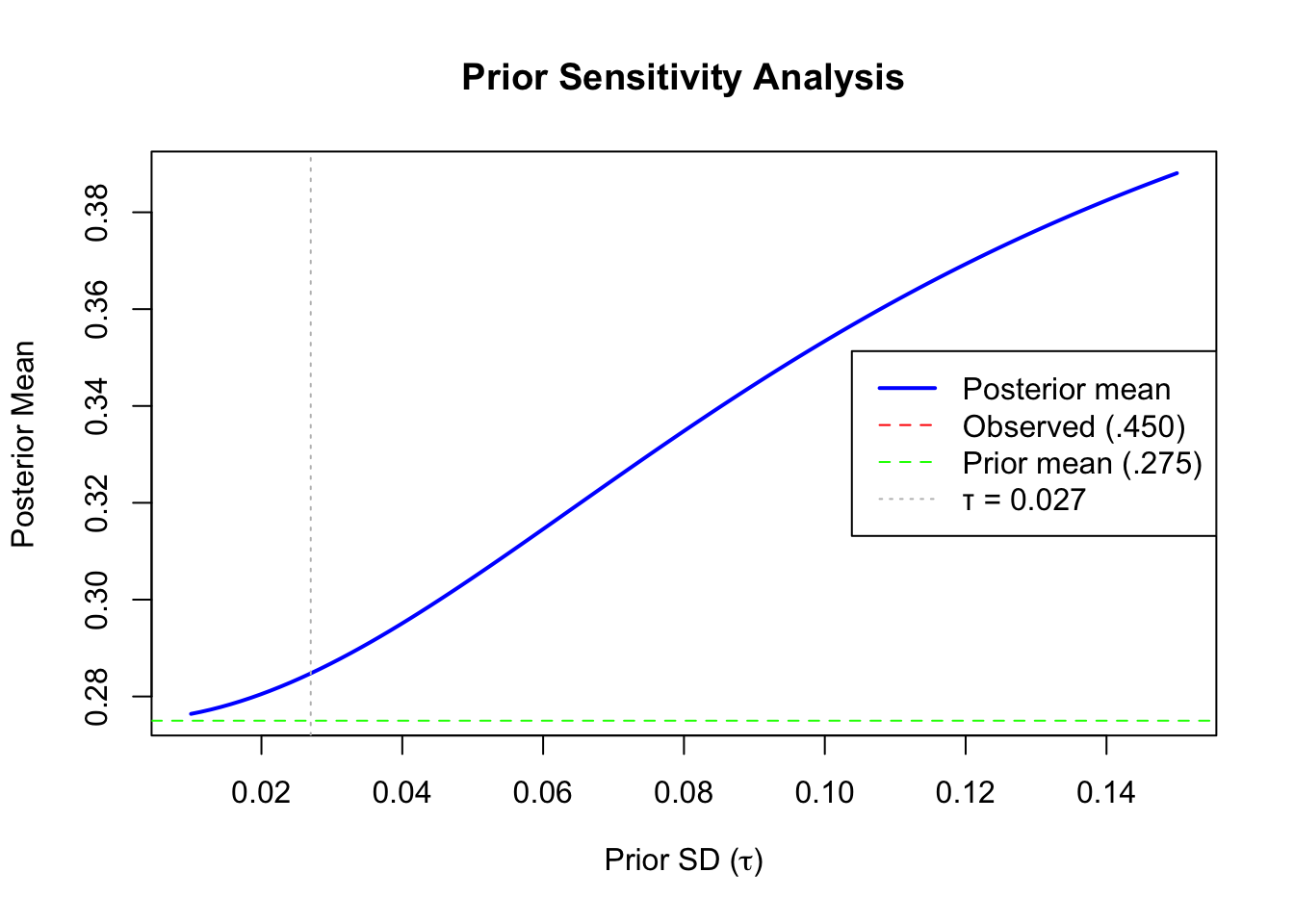
# How does the posterior change with different priors?tau_values <-seq(0.01, 0.15, length.out =100)posterior_means <-sapply(tau_values, function(tau) { B <- sigma^2/ (sigma^2+ tau^2) B * mu + (1- B) * y})plot(tau_values, posterior_means, type ="l", lwd =2, col ="blue",xlab =expression(paste("Prior SD (", tau, ")")),ylab ="Posterior Mean",main ="Prior Sensitivity Analysis")abline(h = y, lty =2, col ="red") # Observed valueabline(h = mu, lty =2, col ="green") # Prior meanabline(v =0.027, lty =3, col ="gray") # Our chosen taulegend("right", c("Posterior mean", "Observed (.450)", "Prior mean (.275)", "τ = 0.027"),col =c("blue", "red", "green", "gray"), lty =c(1, 2, 2, 3), lwd =c(2, 1, 1, 1))
Figure 40.2: Posterior mean as a function of prior standard deviation: with strong priors (small τ), we trust the population average; with weak priors (large τ), we trust José’s data
40.7 When Bayesian Methods Excel
Bayesian approaches are particularly valuable in several contexts. They excel at combining multiple sources of information, allowing you to incorporate prior knowledge, expert opinion, and data from related studies into a single coherent analysis. When working with hierarchical or multilevel data—such as patients grouped within hospitals or students nested within schools—Bayesian hierarchical models naturally capture this structure and allow appropriate borrowing of strength across groups. Bayesian methods are especially useful when working with small samples, where prior information can stabilize estimates that would otherwise be unreliable. The framework also supports sequential updating, where yesterday’s posterior becomes today’s prior as new data arrive, making it natural for adaptive designs and ongoing monitoring studies. Finally, modern MCMC methods enable fitting complex models that would be analytically or computationally intractable using traditional frequentist approaches, opening doors to realistic models of complicated phenomena.
40.8 Computational Bayesian Statistics
For complex models, posteriors don’t have closed-form solutions. Modern Bayesian statistics relies on Markov Chain Monte Carlo (MCMC) methods to sample from posterior distributions.
Popular tools include: - Stan (via rstan or brms packages in R) - JAGS (via rjags package) - PyMC (in Python)
Code
# Example using brms (Bayesian Regression Models using Stan)library(brms)# Fit a Bayesian linear regressionmodel <-brm(formula = weight ~ height,data = my_data,prior =c(prior(normal(0, 10), class ="b"), # Prior on slopeprior(normal(100, 50), class ="Intercept") # Prior on intercept ))# Summarize posterior distributionssummary(model)
40.9 Exercises
Exercise Bay.1: Sally Clark Case - Base Rate Fallacy
In 1999 in England, Sally Clark was convicted of murdering her two infant sons after both were found dead, apparently from Sudden Infant Death Syndrome (SIDS). Expert testimony stated that the chance of two SIDS deaths was 1 in 73 million, calculated as \((1/8500)^2\). What error did this calculation make?
Suppose the probability of a second SIDS case given a first is actually 1/100 (due to genetic factors). What is \(P(\text{two SIDS deaths})\)?
According to Bayes’ theorem, the probability the prosecution wanted was \(P(\text{guilty} \mid \text{two deaths})\), not \(P(\text{two deaths} \mid \text{innocent})\). Assume:
Using a prior of \(N(0, 0.01^2)\) (based on Florida being historically close), calculate the posterior mean and 95% credible interval for the true spread.
How does the posterior change if we use a wider prior (\(\tau = 0.05\))? What about a narrower prior (\(\tau = 0.005\))?
40.10 Summary
Bayes’ theorem provides a principled way to update beliefs based on evidence
The base rate fallacy occurs when prior probabilities are ignored
Bayesian inference treats parameters as random variables with distributions
The posterior combines prior beliefs with observed data
Hierarchical models borrow strength across related observations through shrinkage
Credible intervals have a more intuitive interpretation than confidence intervals
Prior sensitivity analysis checks whether conclusions depend on prior assumptions
Modern Bayesian computation uses MCMC methods implemented in tools like Stan
40.11 Additional Resources
Gelman et al. (2013) - The comprehensive reference for Bayesian data analysis
Kruschke (2014) - Accessible introduction with R examples
McElreath (2020) - Excellent modern treatment with Stan
James et al. (2023) - Connects Bayesian ideas to statistical learning
Gelman, Andrew, John B. Carlin, Hal S. Stern, David B. Dunson, Aki Vehtari, and Donald B. Rubin. 2013. Bayesian Data Analysis. 3rd ed. Boca Raton, FL: CRC Press.
James, Gareth, Daniela Witten, Trevor Hastie, and Robert Tibshirani. 2023. An Introduction to Statistical Learning with Applications in r. 2nd ed. Springer. https://www.statlearning.com.
Kruschke, John K. 2014. Doing Bayesian Data Analysis: A Tutorial with r, JAGS, and Stan. 2nd ed. Boston: Academic Press.
McElreath, Richard. 2020. Statistical Rethinking: A Bayesian Course with Examples in r and Stan. 2nd ed. Boca Raton, FL: CRC Press.
Source Code
# Bayesian Statistics {#sec-bayesian-statistics}```{r}#| echo: false#| message: falselibrary(tidyverse)theme_set(theme_minimal())```## A Different Approach to ProbabilityWhat does it mean when an election forecaster tells us that a candidate has a 90% chance of winning? In classical (frequentist) statistics, probability refers to long-run frequencies of events. A parameter like the true proportion of voters supporting a candidate is a fixed but unknown number—it doesn't make sense to assign it a probability.**Bayesian statistics** takes a different view: probability represents our *degree of belief* about uncertain quantities. Under this framework, we can legitimately say "there is a 90% probability that candidate A will win" because we're expressing our uncertainty about the outcome.This chapter introduces Bayesian thinking and shows how it provides a principled framework for combining prior knowledge with observed data.## Bayes' Theorem: The FoundationBayes' theorem relates conditional probabilities:$$P(A \mid B) = \frac{P(B \mid A) \cdot P(A)}{P(B)}$$This simple equation has profound implications. It tells us how to update our beliefs about $A$ after observing evidence $B$.### A Diagnostic Test ExampleConsider a test for cystic fibrosis with 99% accuracy:$$P(+ \mid D=1) = 0.99 \quad \text{and} \quad P(- \mid D=0) = 0.99$$where $+$ denotes a positive test result and $D$ indicates disease status (1 = has disease, 0 = doesn't).If a randomly selected person tests positive, what is the probability they actually have the disease?The cystic fibrosis rate is approximately 1 in 3,900, so $P(D=1) = 0.00025$.Applying Bayes' theorem:$$\begin{aligned}P(D=1 \mid +) &= \frac{P(+ \mid D=1) \cdot P(D=1)}{P(+)} \\[1em]&= \frac{P(+ \mid D=1) \cdot P(D=1)}{P(+ \mid D=1) \cdot P(D=1) + P(+ \mid D=0) \cdot P(D=0)}\end{aligned}$$Plugging in the numbers:$$P(D=1 \mid +) = \frac{0.99 \times 0.00025}{0.99 \times 0.00025 + 0.01 \times 0.99975} = 0.024$$Despite the test having 99% accuracy, the probability of having the disease given a positive test is only about 2.4%. This counterintuitive result arises because the disease is so rare—most positive tests are false positives from the large healthy population.### Simulation to Verify```{r}set.seed(42)prev <-0.00025N <-100000accuracy <-0.99# Randomly assign disease statusoutcome <-sample(c("Disease", "Healthy"), N, replace =TRUE,prob =c(prev, 1- prev))N_D <-sum(outcome =="Disease")N_H <-sum(outcome =="Healthy")cat("People with disease:", N_D, "\n")cat("Healthy people:", N_H, "\n")# Administer testtest <-vector("character", N)test[outcome =="Disease"] <-sample(c("+", "-"), N_D, replace =TRUE,prob =c(accuracy, 1- accuracy))test[outcome =="Healthy"] <-sample(c("-", "+"), N_H, replace =TRUE,prob =c(accuracy, 1- accuracy))# Resultsconfusion <-table(outcome, test)print(confusion)# Probability of disease given positive testcat("\nP(Disease | Positive test):",round(sum(test =="+"& outcome =="Disease") /sum(test =="+"), 3), "\n")```The simulation confirms our calculation: despite the high test accuracy, most people who test positive are actually healthy because the disease is so rare.::: {.callout-important}## The Base Rate FallacyIgnoring the base rate (prior probability) of a condition leads to dramatically wrong conclusions. This is critical in medical testing, forensic evidence, and any diagnostic situation. Always consider:1. How accurate is the test? (sensitivity, specificity)2. How common is the condition? (base rate/prevalence)3. What population is being tested? (targeted vs. general screening):::## From Bayes' Theorem to Bayesian InferenceBayes' theorem becomes a framework for statistical inference when we apply it to unknown parameters:$$P(\theta \mid \text{data}) = \frac{P(\text{data} \mid \theta) \cdot P(\theta)}{P(\text{data})}$$The components have specific names:| Term | Name | Meaning ||:-----|:-----|:--------|| $P(\theta \mid \text{data})$ | **Posterior** | Updated belief after seeing data || $P(\text{data} \mid \theta)$ | **Likelihood** | Probability of data given parameter || $P(\theta)$ | **Prior** | Initial belief before seeing data || $P(\text{data})$ | **Evidence** | Normalizing constant |The posterior combines what we knew before (prior) with what the data tell us (likelihood).## Hierarchical Models: Shrinkage and Borrowing StrengthOne of Bayesian statistics' most powerful applications is **hierarchical modeling**, where we model variability at multiple levels. This allows us to "borrow strength" across related observations.### A Baseball ExampleConsider José Iglesias, a baseball player who in April 2013 had the following statistics:| Month | At Bats | Hits | AVG ||:------|:--------|:-----|:----|| April | 20 | 9 | .450 |A batting average (AVG) of .450 is extraordinarily high—no player has finished a season above .400 since Ted Williams in 1941. How should we predict José's season-ending average?**The frequentist approach** uses only José's data. With $p = 0.450$ as our estimate and $n = 20$ at bats:$$\text{SE} = \sqrt{\frac{0.450 \times 0.550}{20}} = 0.111$$A 95% confidence interval is $.450 \pm 0.222$, or roughly $.228$ to $.672$. This interval is wide and centered at .450, implying our best guess is that José will break Ted Williams' record.**The Bayesian approach** incorporates what we know about baseball players in general.### The Prior: What Do We Know About Batting Averages?Let's examine batting averages for players with substantial at-bats over recent seasons:```{r}#| label: fig-batting-averages#| fig-cap: "Distribution of batting averages for MLB players with 500+ at-bats (2010-2012)"#| fig-width: 9#| fig-height: 3#| message: false#| warning: falselibrary(Lahman)batting_data <- Batting |>filter(yearID %in%2010:2012) |>mutate(AVG = H / AB) |>filter(AB >500)batting_data |>ggplot(aes(AVG)) +geom_histogram(bins =30, fill ="steelblue", color ="white") +facet_wrap(~yearID) +labs(x ="Batting Average", y ="Count",title ="MLB Batting Averages by Year")# Summary statisticscat("Mean batting average:", round(mean(batting_data$AVG), 3), "\n")cat("SD of batting averages:", round(sd(batting_data$AVG), 3), "\n")```The average player has an AVG around .275 with a standard deviation of about 0.027. José's .450 is over six standard deviations above the mean—an extreme anomaly if taken at face value.### The Hierarchical ModelWe model the data at two levels:**Level 1 (Prior)**: Each player has a "true" batting ability $p$ drawn from a population distribution:$$p \sim N(\mu, \tau^2)$$**Level 2 (Likelihood)**: Given ability $p$, observed performance $Y$ varies due to luck:$$Y \mid p \sim N(p, \sigma^2)$$From the data:- Population mean: $\mu = 0.275$- Population SD: $\tau = 0.027$- Individual sampling error: $\sigma = \sqrt{p(1-p)/n} \approx 0.111$### The Posterior: Combining Prior and DataFor this model, the posterior distribution has a beautiful closed form. The posterior mean is:$$E(p \mid Y = y) = B \cdot \mu + (1-B) \cdot y$$where the **shrinkage factor** $B$ is:$$B = \frac{\sigma^2}{\sigma^2 + \tau^2}$$This is a **weighted average** of the population mean $\mu$ and observed data $y$. The weights depend on:- How much individual variation there is ($\sigma$)- How much population variation there is ($\tau$)When individual uncertainty is high relative to population variation, we "shrink" more toward the population mean.### Applying to José Iglesias```{r}# Parametersmu <-0.275# Population meantau <-0.027# Population SDsigma <-0.111# José's sampling error (from 20 at-bats)y <-0.450# José's observed average# Shrinkage factorB <- sigma^2/ (sigma^2+ tau^2)cat("Shrinkage factor B:", round(B, 3), "\n")# Posterior meanposterior_mean <- B * mu + (1- B) * ycat("Posterior mean (predicted true ability):", round(posterior_mean, 3), "\n")# Posterior standard errorposterior_se <-sqrt(1/ (1/sigma^2+1/tau^2))cat("Posterior SE:", round(posterior_se, 3), "\n")# 95% credible intervalci_lower <- posterior_mean -1.96* posterior_seci_upper <- posterior_mean +1.96* posterior_secat("95% credible interval: [", round(ci_lower, 3), ",", round(ci_upper, 3), "]\n")```The Bayesian estimate "shrinks" José's .450 toward the population average, giving a predicted true ability of about .285. The 95% credible interval is much narrower than the frequentist interval.### The OutcomeHere's how José actually performed through the season:| Month | At Bats | Hits | AVG ||:------|:--------|:-----|:----|| April | 20 | 9 | .450 || May | 26 | 11 | .423 || June | 86 | 34 | .395 || July | 83 | 17 | .205 || August | 85 | 25 | .294 || September | 50 | 10 | .200 || **Total (w/o April)** | **330** | **97** | **.294** |His final average (excluding April) was .294—almost exactly what the Bayesian model predicted! The hierarchical approach correctly recognized that his early performance was partially luck and regressed his prediction toward the population mean.```{r}#| label: fig-shrinkage-illustration#| fig-cap: "Bayesian shrinkage pulls extreme observations toward the population mean"#| fig-width: 8#| fig-height: 5# Visualize shrinkageobservations <-c(0.450, 0.320, 0.260, 0.200)labels <-c("José (Apr)", "Good hitter", "Average", "Struggling")# Calculate posteriors for eachposteriors <- B * mu + (1- B) * observations# Plotplot(1:4, observations, pch =19, cex =2, col ="blue",ylim =c(0.15, 0.50), xlim =c(0.5, 4.5),xaxt ="n", xlab ="", ylab ="Batting Average",main ="Bayesian Shrinkage: Observations → Posteriors")axis(1, at =1:4, labels = labels, las =2)points(1:4, posteriors, pch =17, cex =2, col ="red")arrows(1:4, observations, 1:4, posteriors,length =0.1, col ="gray50", lwd =2)abline(h = mu, lty =2, col ="darkgreen", lwd =2)legend("topright",c("Observed", "Posterior estimate", "Population mean"),pch =c(19, 17, NA), lty =c(NA, NA, 2),col =c("blue", "red", "darkgreen"), pt.cex =1.5)```Notice how the shrinkage is proportional to how extreme the observation is. José's .450 shrinks dramatically, while the average player's .260 barely moves.## Credible Intervals vs. Confidence IntervalsBayesian inference produces **credible intervals** rather than confidence intervals. The interpretation differs:|| Frequentist Confidence Interval | Bayesian Credible Interval ||:--|:--|:--|| Statement | "95% of intervals from repeated sampling would contain the true value" | "There is a 95% probability the true value lies in this interval" || Parameter | Fixed but unknown | Random variable with a distribution || Interpretation | About the procedure | About the parameter |The Bayesian interpretation is often more intuitive: we can directly say "there's a 95% probability the true batting average is between .233 and .337."## Choosing PriorsThe prior distribution encodes what we believe before seeing data. Prior choice is both a strength (incorporating domain knowledge) and a criticism (subjectivity) of Bayesian methods.### Types of PriorsPriors fall along a spectrum of informativeness. **Informative priors** incorporate substantial prior knowledge—for example, a prior for batting average based on historical data might be N(0.275, 0.027²), reflecting that most players hit between .220 and .330. **Weakly informative priors** provide gentle regularization without imposing strong beliefs; a prior of N(0, 10²) for a regression coefficient allows a wide range of values while preferring smaller effects over extremely large ones. Finally, **non-informative** or **diffuse priors** attempt to "let the data speak" by imposing minimal prior constraints—for instance, a uniform prior on [0, 1] for a probability parameter, or an improper prior where P(θ) ∝ 1 across the entire real line.::: {.callout-note}## Empirical BayesWhen we estimate prior parameters from data (as we did with batting averages), this is called **empirical Bayes**. It's a practical compromise: we use the data twice—once to set the prior, once for inference—but it often works well in practice.:::### Prior SensitivityIt's good practice to check whether conclusions depend strongly on prior choice:```{r}#| label: fig-prior-sensitivity#| fig-cap: "Posterior mean as a function of prior standard deviation: with strong priors (small τ), we trust the population average; with weak priors (large τ), we trust José's data"#| fig-width: 7#| fig-height: 5# How does the posterior change with different priors?tau_values <-seq(0.01, 0.15, length.out =100)posterior_means <-sapply(tau_values, function(tau) { B <- sigma^2/ (sigma^2+ tau^2) B * mu + (1- B) * y})plot(tau_values, posterior_means, type ="l", lwd =2, col ="blue",xlab =expression(paste("Prior SD (", tau, ")")),ylab ="Posterior Mean",main ="Prior Sensitivity Analysis")abline(h = y, lty =2, col ="red") # Observed valueabline(h = mu, lty =2, col ="green") # Prior meanabline(v =0.027, lty =3, col ="gray") # Our chosen taulegend("right", c("Posterior mean", "Observed (.450)", "Prior mean (.275)", "τ = 0.027"),col =c("blue", "red", "green", "gray"), lty =c(1, 2, 2, 3), lwd =c(2, 1, 1, 1))```## When Bayesian Methods ExcelBayesian approaches are particularly valuable in several contexts. They excel at **combining multiple sources of information**, allowing you to incorporate prior knowledge, expert opinion, and data from related studies into a single coherent analysis. When working with **hierarchical or multilevel data**—such as patients grouped within hospitals or students nested within schools—Bayesian hierarchical models naturally capture this structure and allow appropriate borrowing of strength across groups. Bayesian methods are especially useful when working with **small samples**, where prior information can stabilize estimates that would otherwise be unreliable. The framework also supports **sequential updating**, where yesterday's posterior becomes today's prior as new data arrive, making it natural for adaptive designs and ongoing monitoring studies. Finally, modern **MCMC methods** enable fitting complex models that would be analytically or computationally intractable using traditional frequentist approaches, opening doors to realistic models of complicated phenomena.## Computational Bayesian StatisticsFor complex models, posteriors don't have closed-form solutions. Modern Bayesian statistics relies on **Markov Chain Monte Carlo (MCMC)** methods to sample from posterior distributions.Popular tools include:- **Stan** (via `rstan` or `brms` packages in R)- **JAGS** (via `rjags` package)- **PyMC** (in Python)```{r}#| eval: false# Example using brms (Bayesian Regression Models using Stan)library(brms)# Fit a Bayesian linear regressionmodel <-brm(formula = weight ~ height,data = my_data,prior =c(prior(normal(0, 10), class ="b"), # Prior on slopeprior(normal(100, 50), class ="Intercept") # Prior on intercept ))# Summarize posterior distributionssummary(model)```## Exercises::: {.callout-note}### Exercise Bay.1: Sally Clark Case - Base Rate Fallacy1. In 1999 in England, Sally Clark was convicted of murdering her two infant sons after both were found dead, apparently from Sudden Infant Death Syndrome (SIDS). Expert testimony stated that the chance of two SIDS deaths was 1 in 73 million, calculated as $(1/8500)^2$. What error did this calculation make?2. Suppose the probability of a second SIDS case given a first is actually 1/100 (due to genetic factors). What is $P(\text{two SIDS deaths})$?3. According to Bayes' theorem, the probability the prosecution wanted was $P(\text{guilty} \mid \text{two deaths})$, not $P(\text{two deaths} \mid \text{innocent})$. Assume: - $P(\text{two deaths} \mid \text{guilty}) = 0.50$ - $P(\text{guilty}) = 1/1,000,000$ (rate of child-murdering parents) - $P(\text{two natural deaths}) = 1/8500 \times 1/100 = 1.2 \times 10^{-5}$ Calculate $P(\text{guilty} \mid \text{two deaths})$.:::::: {.callout-note}### Exercise Bay.2: Bayesian Election Polling4. Consider a Bayesian model for Florida election polling:```{r}#| eval: falselibrary(dslabs)data(polls_us_election_2016)polls <- polls_us_election_2016 |>filter(state =="Florida"& enddate >="2016-11-04") |>mutate(spread = rawpoll_clinton/100- rawpoll_trump/100)# Calculate average spread and SEresults <- polls |>summarize(avg =mean(spread),se =sd(spread) /sqrt(n()) )``` Using a prior of $N(0, 0.01^2)$ (based on Florida being historically close), calculate the posterior mean and 95% credible interval for the true spread.5. How does the posterior change if we use a wider prior ($\tau = 0.05$)? What about a narrower prior ($\tau = 0.005$)?:::## Summary- **Bayes' theorem** provides a principled way to update beliefs based on evidence- The **base rate fallacy** occurs when prior probabilities are ignored- **Bayesian inference** treats parameters as random variables with distributions- The **posterior** combines prior beliefs with observed data- **Hierarchical models** borrow strength across related observations through shrinkage- **Credible intervals** have a more intuitive interpretation than confidence intervals- **Prior sensitivity analysis** checks whether conclusions depend on prior assumptions- Modern Bayesian computation uses **MCMC** methods implemented in tools like Stan## Additional Resources- @gelman2013bayesian - The comprehensive reference for Bayesian data analysis- @kruschke2014doing - Accessible introduction with R examples- @mcelreath2020statistical - Excellent modern treatment with Stan- @james2023islr - Connects Bayesian ideas to statistical learning