11  Foundations of Probability

11.1 Why Probability Matters

In games of chance, probability has a very intuitive definition. We know what it means that the chance of a pair of dice coming up seven is 1 in 6. However, probability is used much more broadly today, with the word commonly appearing in everyday language. Google’s auto-complete of “What are the chances of” gives us: “having twins”, “rain today”, “getting struck by lightning”, and “getting cancer”. One goal of this chapter is to help us understand how probability is useful to understand and describe real-world events when performing data analysis.

Because knowing how to compute probabilities gives you an edge in games of chance, throughout history many smart individuals—including famous mathematicians such as Cardano, Fermat, and Pascal—spent time and energy thinking through the math of these games. As a result, Probability Theory was born. Probability continues to be highly useful in modern games of chance. For example, in poker, we can compute the probability of winning a hand based on the cards on the table. Casinos rely on probability theory to develop games that almost certainly guarantee a profit.

Probability theory is useful in many other contexts and, in particular, in areas that depend on data affected by chance in some way. All of the other chapters in this part build upon probability theory. Knowledge of probability is therefore indispensable for data science.

11.2 Two Interpretations of Probability

There are two main ways to think about what probability means.

The frequentist interpretation views probability as mathematically convenient approximations to long-run relative frequencies. If we say the probability of heads when flipping a fair coin is 0.5, we mean that if we flipped the coin many, many times, about half the flips would come up heads. This interpretation grounds probability in observable, repeatable phenomena.

The subjective (Bayesian) interpretation views probability as a measure of belief or uncertainty. A probability statement expresses the opinion of some individual regarding how certain an event is to occur, given their current information. This interpretation allows us to assign probabilities to one-time events and to update beliefs as we gather evidence.

Both interpretations have their uses, and modern statistics draws on both perspectives. For now, the frequentist interpretation provides good intuition for the concepts we will develop.

11.3 Random Variables and Sample Spaces

A random variable is a quantity that can take on different values with different probabilities. The outcome of a coin flip, the number of bacterial colonies on a plate, and the expression level of a gene are all random variables.

The sample space of a random variable is the set of all possible values it can take. For a coin flip, the sample space is {Heads, Tails}. For a die roll, it is {1, 2, 3, 4, 5, 6}. For the concentration of a protein, it might be any non-negative real number.

A probability distribution describes how likely each value in the sample space is:

• For discrete random variables (those that take distinct values), we use a probability mass function that gives the probability of each possible value
• For continuous random variables (those that can take any value in a range), we use a probability density function from which probabilities are calculated by integration

One fundamental rule: the probabilities across the entire sample space must sum (or integrate) to 1. Something from the sample space must happen.

11.4 Discrete Probability

We start by covering some basic principles related to categorical data. This subset of probability is referred to as discrete probability. It will help us understand the probability theory we will later introduce for numeric and continuous data, which is much more common in data science applications.

Relative Frequency

A precise definition of probability can be given by noting all possible outcomes and counting how many satisfy the condition for our event. For example, if we have 2 red beads and 3 blue beads inside an urn and we pick one at random, what is the probability of picking a red one?

Our intuition tells us that the answer is 2/5 or 40%. There are five possible outcomes, of which two satisfy the condition necessary for the event “pick a red bead”. Since each of the five outcomes has the same chance of occurring, we conclude that the probability is 0.4 for red and 0.6 for blue.

A more tangible way to think about the probability of an event is as the proportion of times the event occurs when we repeat the experiment an infinite number of times, independently, and under the same conditions.

Notation

We use the notation \(\mbox{Pr}(A)\) to denote the probability of event \(A\) happening. We use the very general term event to refer to things that can happen when something occurs by chance. In our previous example, the event was “picking a red bead”. In a political poll in which we call 100 likely voters at random, an example of an event is “calling 48 Democrats and 52 Republicans”.

In data science applications, we will often deal with continuous variables. These events will often be things like “is this person taller than 6 feet”. In this case, we write events in a more mathematical form: \(X \geq 6\).

Probability Distributions for Categorical Data

If we know the relative frequency of the different categories, defining a distribution for categorical outcomes is straightforward. We simply assign a probability to each category. In cases that can be thought of as beads in an urn, for each bead type, their proportion defines the distribution.

If we are randomly calling likely voters from a population that is 44% Democrat, 44% Republican, 10% undecided, and 2% Green Party, these proportions define the probability for each group:

Group	Probability
Republican	0.44
Democrat	0.44
Undecided	0.10
Green	0.02

11.5 Distribution Moments and Parameters

Probability distributions can be characterized by their moments—metrics that describe the shape of the distribution. The first four moments correspond to important properties:

1. Mean (\(\mu\)) - the center or expected value
2. Variance (\(\sigma^2\)) - the spread or dispersion
3. Skewness - the asymmetry of the distribution
4. Kurtosis - the “tailedness” or peakedness

For a discrete random variable X, the expected value (mean) is:

\[E[X] = \sum_{\text{all } x} x \cdot P(X = x) = \mu\]

The variance measures dispersion around the mean:

\[\text{Var}(X) = E[(X - \mu)^2] = \sigma^2\]

These parameters are crucial because they describe real properties of the systems we study. In biology, for example, the mean height of a population tells us about the typical value, while the variance tells us about the diversity of heights among individuals.

11.6 Monte Carlo Simulations

Computers provide a way to actually perform random experiments. Random number generators permit us to mimic the process of picking at random. An example is the sample function in R.

First, we use the function rep to generate the urn:

beads <- rep(c("red", "blue"), times = c(2, 3))
beads

[1] "red"  "red"  "blue" "blue" "blue"

Then use sample to pick a bead at random:

sample(beads, 1)

[1] "red"

This line of code produces one random outcome. We want to repeat this experiment a large enough number of times to make the results practically equivalent to repeating forever. This is an example of a Monte Carlo simulation.

To perform our first Monte Carlo simulation, we use the replicate function, which permits us to repeat the same task any number of times. Here, we repeat the random event B = 10,000 times:

set.seed(1986)  # For reproducibility
B <- 10000
events <- replicate(B, sample(beads, 1))

We can now see if our definition actually agrees with this Monte Carlo simulation approximation:

tab <- table(events)
prop.table(tab)

events
  blue    red 
0.6014 0.3986 

The numbers above are the estimated probabilities provided by this Monte Carlo simulation. Statistical theory tells us that as \(B\) gets larger, the estimates get closer to 3/5 = 0.6 and 2/5 = 0.4.

With and Without Replacement

The function sample has an argument that permits us to pick more than one element from the urn. By default, this selection occurs without replacement: after a bead is selected, it is not put back in the bag.

sample(beads, 5)

[1] "blue" "red"  "blue" "red"  "blue"

This results in rearrangements that always have three blue and two red beads because we can’t select more beads than exist.

However, we can sample with replacement: return the bead back to the urn after selecting it:

events <- sample(beads, B, replace = TRUE)
prop.table(table(events))

events
 blue   red 
0.601 0.399 

Not surprisingly, we get results very similar to those previously obtained with replicate.

11.7 The Bernoulli Distribution

The simplest probability distribution describes a single event with two possible outcomes—success or failure, yes or no, heads or tails. This is the Bernoulli distribution.

Consider flipping a fair coin once:

\[P(X = \text{Head}) = \frac{1}{2} = 0.5 = p\]

And the probability of tails is:

\[P(X = \text{Tail}) = \frac{1}{2} = 0.5 = 1 - p = q\]

If the coin is not fair, \(p\) might differ from 0.5, but the probabilities still sum to 1:

\[p + (1-p) = 1\]

This same framework applies to any binary outcome: whether a patient responds to treatment, whether an allele is inherited from a parent, or whether a product passes quality control.

# Flip a coin 1000 times
set.seed(42)
flips <- rbinom(1000, 1, 0.5)

barplot(table(flips) / 1000,
        names.arg = c("Tails", "Heads"),
        ylab = "Probability",
        ylim = c(0, 0.75),
        col = "steelblue",
        main = "Estimated Bernoulli Distribution")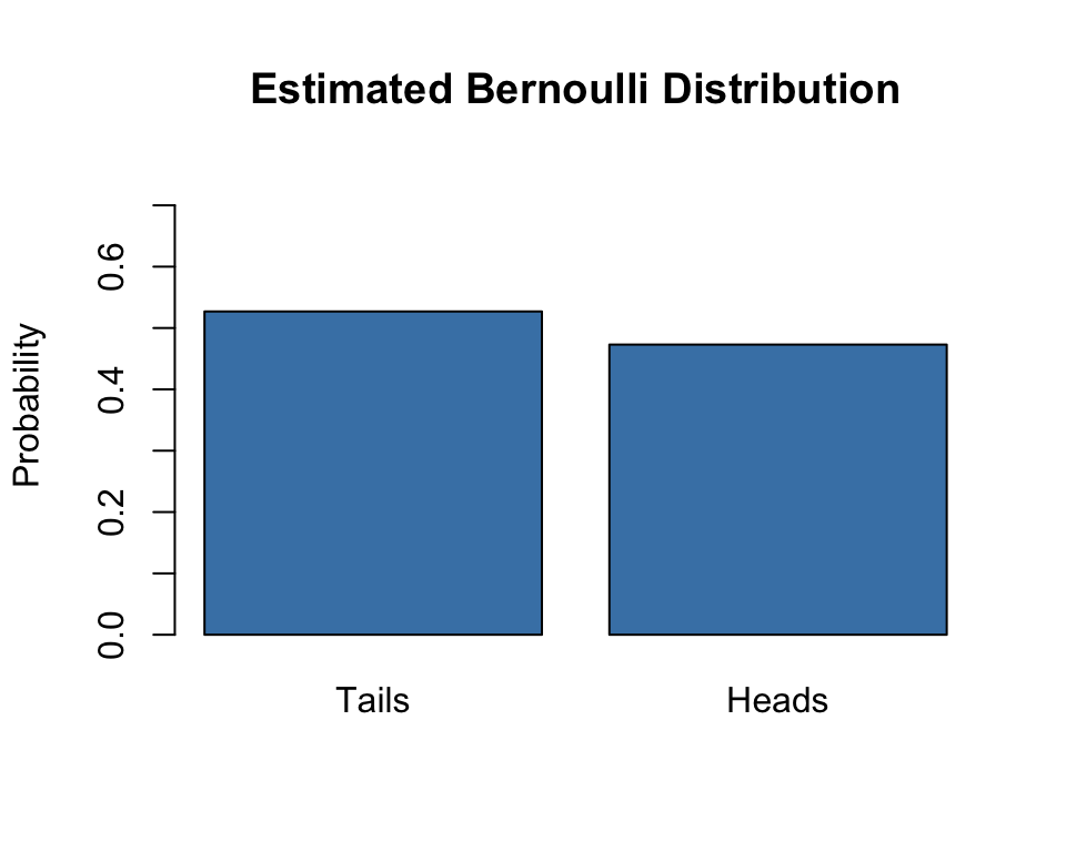

Figure 11.1: Simulated Bernoulli distribution from 1000 coin flips showing approximately equal probability for heads and tails

11.8 Probability Rules

Two fundamental rules govern how probabilities combine. Most probability distributions can be built up from these simple rules.

The AND Rule (Multiplication)

The probability that two independent events both occur is the product of their individual probabilities. If you flip a coin twice:

\[P(\text{First = Head AND Second = Head}) = p \times p = p^2\]

More generally, for independent events A and B:

\[P(A \text{ and } B) = P(A) \times P(B)\]

For a fair coin with \(p = 0.5\):

• \(P(\text{HH}) = 0.5 \times 0.5 = 0.25\)
• \(P(\text{HT}) = 0.5 \times 0.5 = 0.25\)
• \(P(\text{TH}) = 0.5 \times 0.5 = 0.25\)
• \(P(\text{TT}) = 0.5 \times 0.5 = 0.25\)

The OR Rule (Addition)

The probability that at least one of two mutually exclusive events occurs is the sum of their probabilities:

\[P(A \text{ or } B) = P(A) + P(B) - P(A \text{ and } B)\]

For mutually exclusive events (those that cannot both occur), the intersection is empty:

\[P(A \text{ or } B) = P(A) + P(B)\]

The probability of getting exactly one head in two flips (either HT or TH):

\[P(\text{one head}) = P(\text{HT}) + P(\text{TH}) = 0.25 + 0.25 = 0.5\]

Multiplication Rule Under Independence

When events are independent, the multiplication rule simplifies:

\[P(A \text{ and } B \text{ and } C) = P(A) \times P(B) \times P(C)\]

But we must be careful—assuming independence can result in very different and incorrect probability calculations when we don’t actually have independence.

Independence Matters

Imagine a court case where the suspect was described as having a mustache and a beard. The defendant has both, and the prosecution brings in an “expert” who testifies that 1/10 men have beards and 1/5 have mustaches, concluding that only \(1/10 \times 1/5 = 0.02\) have both.

But to multiply like this we need to assume independence! If the conditional probability of a man having a mustache given that he has a beard is 0.95, then the correct probability is much higher: \(1/10 \times 0.95 = 0.095\).

11.9 Independence

We say two events are independent if the outcome of one does not affect the other. The classic example is coin tosses. Every time we toss a fair coin, the probability of seeing heads is 1/2 regardless of what previous tosses have revealed. The same is true when we pick beads from an urn with replacement.

Many examples of events that are not independent come from card games. When we deal the first card, the probability of getting a King is 1/13 since there are thirteen possibilities. Now if we deal a King for the first card and don’t replace it into the deck, the probability of a second card being a King is only 3/51. These events are not independent: the first outcome affected the next one.

# Demonstrate non-independence with sequential draws
set.seed(1)
x <- sample(beads, 5)
x[1:4]  # First four draws

[1] "red"  "blue" "blue" "blue"

x[5]    # If first four are blue, the fifth must be...

[1] "red"

If you have to guess the color of the first bead, you would predict blue since blue has a 60% chance. But if you know the first four were blue, the probability of the fifth being red is now 100%, not 40%. The events are not independent, so the probabilities change.

11.10 Conditional Probabilities

When events are not independent, conditional probabilities are useful. The conditional probability \(P(B|A)\) is the probability of B given that A has occurred:

\[P(\text{Card 2 is a King} \mid \text{Card 1 is a King}) = \frac{3}{51}\]

We use the \(\mid\) as shorthand for “given that” or “conditional on”.

When two events A and B are independent:

\[P(A \mid B) = P(A)\]

This is the mathematical definition of independence: the fact that B happened does not affect the probability of A happening.

The general multiplication rule relates joint and conditional probability:

\[P(A \text{ and } B) = P(A) \times P(B \mid A)\]

This can be extended to more events:

\[P(A \text{ and } B \text{ and } C) = P(A) \times P(B \mid A) \times P(C \mid A \text{ and } B)\]

11.11 Bayes’ Theorem

Rearranging the multiplication rule yields Bayes’ theorem, a cornerstone of probabilistic reasoning:

\[P(A|B) = \frac{P(B|A) \times P(A)}{P(B)}\]

Bayes’ theorem tells us how to update our beliefs about A after observing B. In Bayesian statistics, this is written as:

\[P(\theta|d) = \frac{P(d|\theta) \times P(\theta)}{P(d)}\]

where:

• \(P(\theta|d)\) = posterior probability distribution
• \(P(d|\theta)\) = likelihood function for \(\theta\)
• \(P(\theta)\) = prior probability distribution
• \(P(d)\) = marginal likelihood (normalizing constant)

11.12 Likelihood vs. Probability

A subtle but important distinction exists between probability and likelihood.

Probability is the chance of observing particular data given a model or parameter value. If we know a coin has \(p = 0.5\), what is the probability of observing 7 heads in 10 flips?

Likelihood is how well a parameter value explains observed data. Given that we observed 7 heads in 10 flips, how likely is it that the true probability is \(p = 0.5\) versus \(p = 0.7\)?

Mathematically, the likelihood function uses the same formula as probability, but we think of it differently:

\[L(\text{parameter} | \text{data}) = P(\text{data} | \text{parameter})\]

Maximum likelihood estimation finds the parameter value that makes the observed data most probable—the value that maximizes the likelihood function.

11.13 Combinations and Permutations

For more complicated probability calculations, we need to count possibilities systematically. The gtools package provides useful functions.

Permutations (Order Matters)

A permutation is an arrangement where order matters. For any list of size n, the permutations function computes all different arrangements when selecting r items:

# All ways to arrange 2 items from {1, 2, 3}
permutations(3, 2)

     [,1] [,2]
[1,]    1    2
[2,]    1    3
[3,]    2    1
[4,]    2    3
[5,]    3    1
[6,]    3    2

Notice that order matters: 3,1 is different than 1,3. Also, (1,1), (2,2), and (3,3) do not appear because once we pick a number, it can’t appear again.

Combinations (Order Doesn’t Matter)

A combination is a selection where order doesn’t matter:

combinations(3, 2)

     [,1] [,2]
[1,]    1    2
[2,]    1    3
[3,]    2    3

The outcome (2,1) doesn’t appear because (1,2) already represents the same combination.

Example: Blackjack

Let’s compute the probability of getting a “Natural 21” in Blackjack—an Ace and a face card in the first two cards:

# Build a deck
suits <- c("Diamonds", "Clubs", "Hearts", "Spades")
numbers <- c("Ace", "Deuce", "Three", "Four", "Five", "Six", "Seven",
             "Eight", "Nine", "Ten", "Jack", "Queen", "King")
deck <- expand.grid(number = numbers, suit = suits)
deck <- paste(deck$number, deck$suit)

# Define aces and face cards
aces <- paste("Ace", suits)
facecard <- c("King", "Queen", "Jack", "Ten")
facecard <- expand.grid(number = facecard, suit = suits)
facecard <- paste(facecard$number, facecard$suit)

# All possible two-card hands (order doesn't matter)
hands <- combinations(52, 2, v = deck)

# Probability of Natural 21
mean((hands[,1] %in% aces & hands[,2] %in% facecard) |
     (hands[,2] %in% aces & hands[,1] %in% facecard))

[1] 0.04826546

11.14 Classic Examples

The Monty Hall Problem

In the game show “Let’s Make a Deal,” contestants pick one of three doors. Behind one door is a car; behind the others are goats. After you pick a door, Monty Hall opens one of the remaining doors to reveal a goat. Then he asks: “Do you want to switch doors?”

Intuition suggests it shouldn’t matter—you’re choosing between two doors, so shouldn’t the probability be 50-50? Let’s use Monte Carlo simulation:

B <- 10000
monty_hall <- function(strategy) {
  doors <- as.character(1:3)
  prize <- sample(c("car", "goat", "goat"))
  prize_door <- doors[prize == "car"]
  my_pick <- sample(doors, 1)
  show <- sample(doors[!doors %in% c(my_pick, prize_door)], 1)

  if (strategy == "stick") {
    choice <- my_pick
  } else {
    choice <- doors[!doors %in% c(my_pick, show)]
  }
  choice == prize_door
}

stick_wins <- replicate(B, monty_hall("stick"))
switch_wins <- replicate(B, monty_hall("switch"))

cat("Probability of winning when sticking:", mean(stick_wins), "\n")

Probability of winning when sticking: 0.3365 

cat("Probability of winning when switching:", mean(switch_wins), "\n")

Probability of winning when switching: 0.6643 

Switching doubles your chances! The key insight: when you first pick, you have a 1/3 chance of being right. Monty’s reveal doesn’t change that. Since the probability the car is behind one of the other doors was 2/3, and Monty showed you which one doesn’t have it, switching gives you that 2/3 probability.

The Birthday Problem

In a room with 50 people, what’s the probability that at least two share a birthday?

# Monte Carlo simulation
B <- 10000
same_birthday <- function(n) {
  bdays <- sample(1:365, n, replace = TRUE)
  any(duplicated(bdays))
}

results <- replicate(B, same_birthday(50))
cat("Probability with 50 people:", mean(results), "\n")

Probability with 50 people: 0.9701 

# How does this change with group size?
compute_prob <- function(n, B = 10000) {
  results <- replicate(B, same_birthday(n))
  mean(results)
}

n <- seq(1, 60)
prob <- sapply(n, compute_prob)
qplot(n, prob, geom = "line") +
  geom_hline(yintercept = 0.5, linetype = "dashed", color = "red") +
  labs(x = "Group Size", y = "Probability of Shared Birthday",
       title = "The Birthday Problem")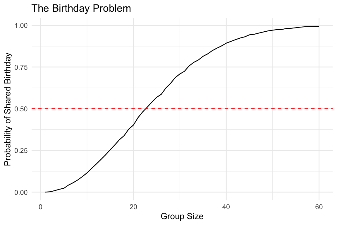

Figure 11.2: The probability of at least two people sharing a birthday increases rapidly with group size, exceeding 50% at just 23 people

With just 23 people, there’s already a 50% chance of a shared birthday! People tend to underestimate these probabilities because they think about the probability that someone shares their birthday, not the probability that any two people share a birthday.

We can also compute this exactly using the multiplication rule:

# Probability that all n people have UNIQUE birthdays
exact_prob <- function(n) {
  prob_unique <- seq(365, 365 - n + 1) / 365
  1 - prod(prob_unique)
}

eprob <- sapply(n, exact_prob)
cat("Exact probability with 50 people:", exact_prob(50), "\n")

Exact probability with 50 people: 0.9703736 

11.15 Covariance and Correlation

When two variables are not independent, they share information—knowing one tells you something about the other. This shared information is quantified by covariance, a measure of how two variables vary together.

If high values of X tend to occur with high values of Y (and low with low), the covariance is positive. If high values of X tend to occur with low values of Y, the covariance is negative. If there is no relationship, the covariance is near zero.

Correlation is covariance standardized to fall between -1 and 1, making it easier to interpret. A correlation of 1 means perfect positive linear relationship; -1 means perfect negative linear relationship; 0 means no linear relationship.

These concepts will become central when we discuss regression and other methods for relating variables to each other.

11.16 How Large is “Large Enough” for Monte Carlo?

The theory described here requires repeating experiments over and over forever. In practice, we can’t do this. In the examples above, we used \(B = 10,000\) Monte Carlo experiments and it turned out to provide accurate estimates.

One practical approach is to check for the stability of the estimate:

B_values <- 10^seq(1, 5, len = 100)
compute_prob_B <- function(B, n = 25) {
  same_day <- replicate(B, same_birthday(n))
  mean(same_day)
}

prob <- sapply(B_values, compute_prob_B)
qplot(log10(B_values), prob, geom = "line") +
  geom_hline(yintercept = exact_prob(25), color = "red", linetype = "dashed") +
  labs(x = "log10(Number of Simulations)", y = "Estimated Probability",
       title = "Monte Carlo Convergence")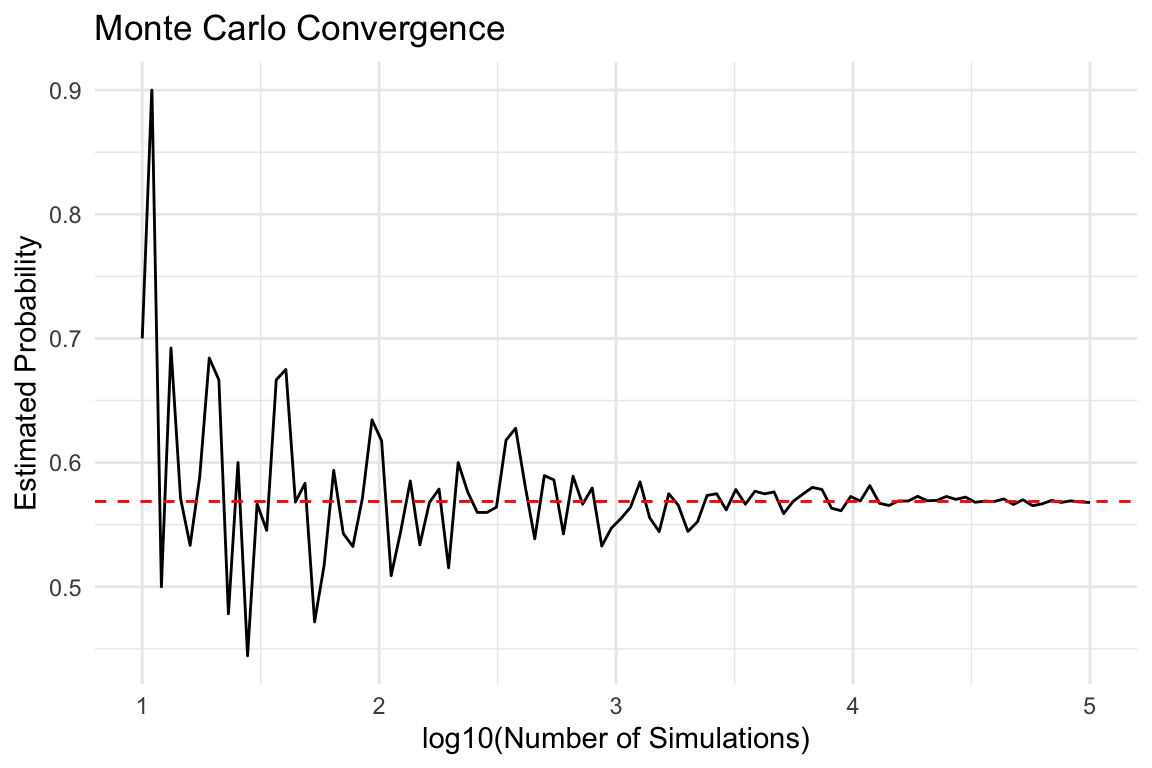

Figure 11.3: Monte Carlo estimates converge to the true probability (red dashed line) as the number of simulations increases

The values start to stabilize (vary less than 0.01) around 1000 simulations. The exact probability is shown in red.

11.17 Summary

This chapter introduced the language of probability:

• Random variables can take different values with different probabilities
• The sample space contains all possible outcomes
• Probability distributions describe how likely each outcome is
• The AND rule (multiply) and OR rule (add) combine probabilities
• Independence means one event doesn’t affect another’s probability
• Conditional probability describes probability given other information
• Bayes’ theorem updates beliefs based on new evidence
• Monte Carlo simulations estimate probabilities through repeated random sampling
• Classic problems like Monty Hall and birthdays reveal counterintuitive probability results

Understanding these foundations is essential for all statistical inference that follows.

11.18 Practice Exercises

Exercise P.1: Simulating Coin Flips

Use R to simulate coin flips:

set.seed(123)

1. Simulate 100 fair coin flips using rbinom() or sample()
2. Calculate the proportion of heads
3. Repeat with 1000 and 10000 flips—how does the proportion change?
4. Create a histogram of results from many simulations

# Simulate coin flips
n_flips <- 1000
flips <- rbinom(n_flips, size = 1, prob = 0.5)
mean(flips)  # Proportion of heads (1s)

# Or using sample
flips <- sample(c("H", "T"), n_flips, replace = TRUE)
mean(flips == "H")

Exercise P.2: Binomial Distribution

Explore the binomial distribution:

1. Use rbinom() to simulate 1000 experiments, each with 20 coin flips
2. Create a histogram of the number of heads per experiment
3. What is the most common outcome? Does this match your expectation?
4. Change the probability to simulate an unfair coin
5. How does the distribution change with 200 or 2000 flips per experiment?

# 1000 experiments, 20 flips each, fair coin
set.seed(42)
results <- rbinom(1000, size = 20, prob = 0.5)
hist(results, breaks = 20, col = "steelblue",
     main = "Number of Heads in 20 Flips",
     xlab = "Number of Heads")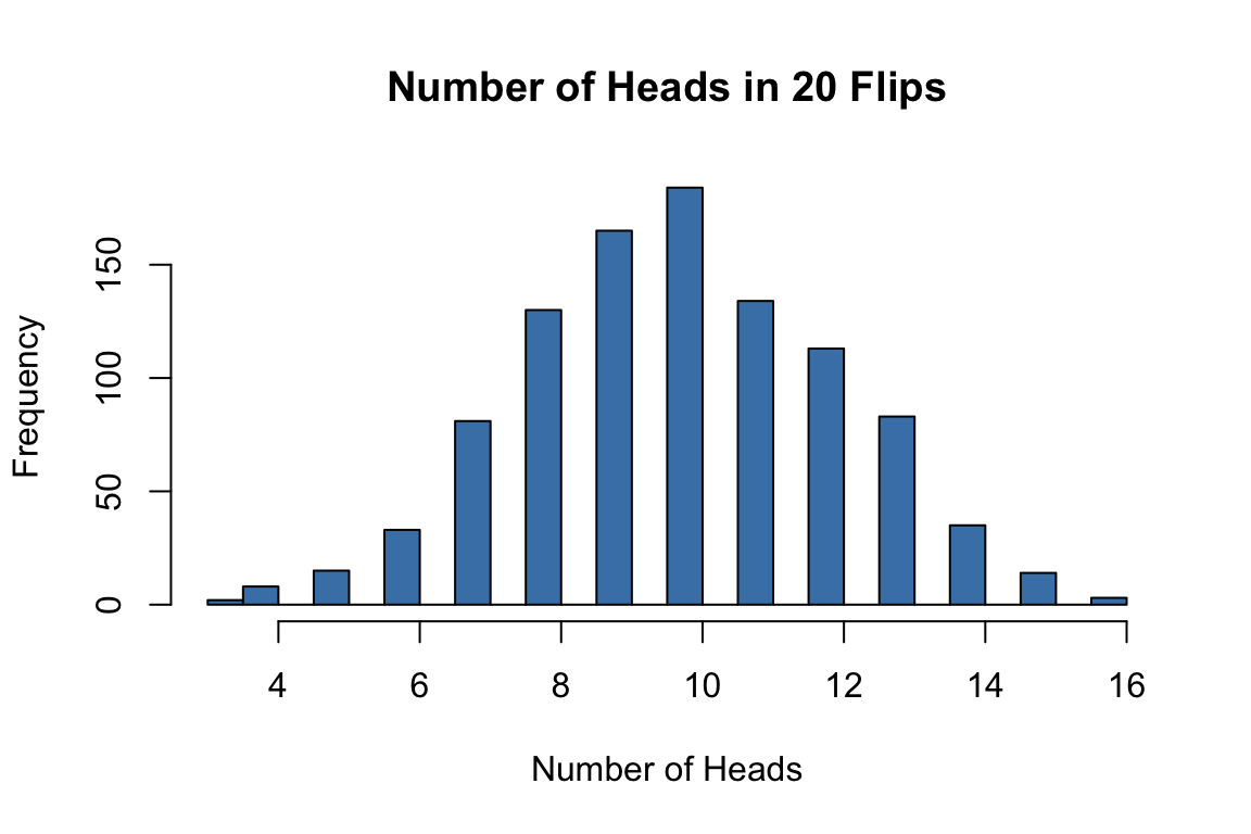

Figure 11.4: Distribution of heads from 1000 simulated experiments of 20 coin flips each

Exercise P.3: The Birthday Problem

Use Monte Carlo simulation to explore the birthday problem:

1. Write a function that simulates whether any two people in a group share a birthday
2. Estimate the probability for groups of size 10, 23, and 50
3. Plot the probability as a function of group size
4. At what group size does the probability exceed 50%?

# Birthday simulation function
same_birthday <- function(n, B = 10000) {
  matches <- replicate(B, {
    birthdays <- sample(1:365, n, replace = TRUE)
    any(duplicated(birthdays))
  })
  mean(matches)
}

# Test for different group sizes
sizes <- 2:50
probs <- sapply(sizes, same_birthday)
plot(sizes, probs, type = "l",
     xlab = "Group Size", ylab = "Probability of Shared Birthday")
abline(h = 0.5, col = "red", lty = 2)

Exercise P.4: Conditional Probability

Explore conditional probability with card simulations:

1. Create a virtual deck of 52 cards
2. Calculate the probability of drawing a King
3. Given that the first card drawn is a King, what is the probability the second card is also a King?
4. Use simulation to verify your calculation

Exercise P.5: The Monty Hall Problem

Simulate the Monty Hall problem:

1. Write a function that simulates one round of the game
2. Compare the win rate when you stick versus when you switch
3. Run 10,000 simulations for each strategy
4. Does switching really double your chances?

11.19 Additional Resources

• Irizarry (2019) - A gitbook by a statistician with excellent introductions to key topics in statistical inference
• Logan (2010) - A comprehensive introduction to R for statistical analysis
• For a detailed reference of common probability distributions, see Chapter 50

Irizarry, Rafael A. 2019. Introduction to Data Science. Self-published. https://rafalab.github.io/dsbook/.

Logan, Murray. 2010. Biostatistical Design and Analysis Using r. Wiley-Blackwell.