16 Hypothesis Testing

16.1 What is a Hypothesis?

A hypothesis is a statement of belief about the world—a claim that can be evaluated with data. In statistics, we formalize hypothesis testing as a framework for using data to decide between competing claims.

The null hypothesis ($H_0$) represents a default position, typically stating that there is no effect, no difference, or no relationship. The alternative hypothesis ($H_A$) represents what we would conclude if we reject the null—typically that there is an effect, difference, or relationship.

For example, consider testing whether an amino acid substitution changes the catalytic rate of an enzyme:

$H_0$: The substitution does not change the catalytic rate
$H_A$: The substitution does change the catalytic rate

The alternative hypothesis might be directional (the substitution increases the rate) or non-directional (the substitution changes the rate, in either direction). This distinction affects how we calculate p-values.

16.2 The Logic of Hypothesis Testing

Hypothesis testing follows a specific logic. We assume the null hypothesis is true and ask: how likely would we be to observe data as extreme as what we actually observed? If this probability is very small, we conclude that the null hypothesis is unlikely to be true and reject it in favor of the alternative.

This framework naturally raises several key questions. What is the probability that we might reject a true null hypothesis, committing a false positive error? Conversely, what is the probability that we might fail to reject a false null hypothesis, missing a real effect? How do we decide when the evidence is strong enough to reject the null hypothesis? And perhaps most subtly, what can we legitimately conclude when we fail to reject the null—does this mean we’ve proven it true, or merely that we lack sufficient evidence against it?

16.3 Type I and Type II Errors

Two types of mistakes are possible in hypothesis testing.

Figure 16.1: Type I and Type II errors in hypothesis testing

A Type I error occurs when we reject a true null hypothesis—concluding there is an effect when there is not. The probability of a Type I error is denoted $\alpha$ and is called the significance level. By convention, $\alpha$ is often set to 0.05, meaning we accept a 5% chance of falsely rejecting a true null.

Figure 16.2: R.A. Fisher’s original 1926 paper “The Arrangement of Field Experiments” where he proposed the 0.05 significance threshold. Fisher wrote that results reaching “the 5 per cent. point” provide “reasonable grounds for calling the result significant.” This arbitrary but practical convention has shaped statistical practice for nearly a century.

A Type II error occurs when we fail to reject a false null hypothesis—concluding there is no effect when there actually is one. The probability of a Type II error is denoted $\beta$.

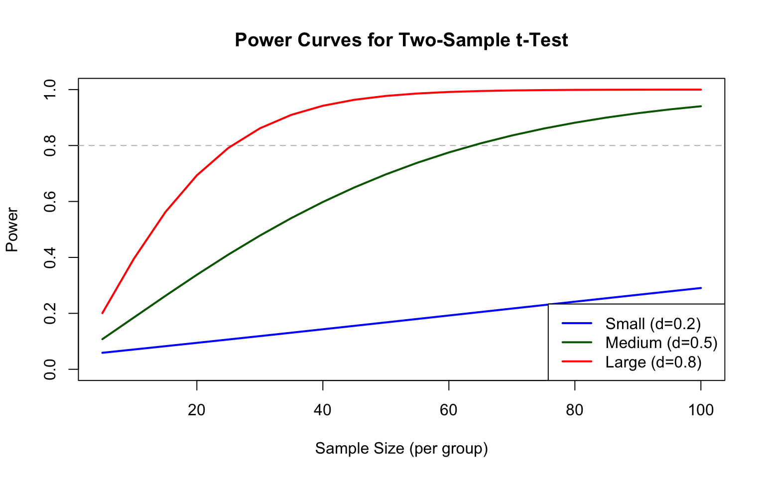
Power is the probability of correctly rejecting a false null hypothesis: Power = $1 - \beta$. Power depends on the effect size (how big the true effect is), sample size, significance level, and variability in the data.

	$H_0$ True	$H_0$ False
Reject $H_0$	Type I Error ($\alpha$)	Correct Decision (Power)
Fail to Reject $H_0$	Correct Decision	Type II Error ($\beta$)

Understanding Statistical Power

Power analysis is essential for designing experiments that can actually detect effects of interest. A study with low power is unlikely to find real effects even when they exist—wasting resources and potentially leading to incorrect conclusions.

Several key factors determine statistical power. Effect size matters fundamentally—larger effects are easier to detect than subtle ones. Sample size directly affects power because more data provides more information about the true state of nature. The chosen significance level ($\alpha$) creates a trade-off: higher $\alpha$ increases power to detect true effects but also increases the Type I error rate. Finally, variability in the data affects how clearly we can see signals; less noise makes true effects easier to detect, while high variability obscures even substantial effects.

For a two-sample t-test, the relationship between these factors can be expressed approximately as:

\[\text{Power} \approx \Phi\left(\frac{|\mu_1 - \mu_2|}{\sigma}\sqrt{\frac{n}{2}} - z_{1-\alpha/2}\right)\]

where $\Phi$ is the standard normal CDF, and $z_{1-\alpha/2}$ is the critical value.

Code

# Visualize how power depends on effect size and sample size
library(pwr)

# Power curves for different effect sizes
effect_sizes <- c(0.2, 0.5, 0.8)  # Cohen's d: small, medium, large
sample_sizes <- seq(5, 100, by = 5)

par(mfrow = c(1, 1))
colors <- c("blue", "darkgreen", "red")

plot(NULL, xlim = c(5, 100), ylim = c(0, 1),
     xlab = "Sample Size (per group)", ylab = "Power",
     main = "Power Curves for Two-Sample t-Test")
abline(h = 0.8, lty = 2, col = "gray")

for (i in 1:3) {
  powers <- sapply(sample_sizes, function(n) {
    pwr.t.test(n = n, d = effect_sizes[i], sig.level = 0.05, type = "two.sample")$power
  })
  lines(sample_sizes, powers, col = colors[i], lwd = 2)
}

legend("bottomright",
       legend = c("Small (d=0.2)", "Medium (d=0.5)", "Large (d=0.8)"),
       col = colors, lwd = 2)

Figure 16.3: Statistical power increases with sample size and effect size; the dashed line indicates the common 80% power threshold

A Priori Power Analysis

Before conducting an experiment, power analysis helps determine the necessary sample size. The question is: “How many observations do I need to have an 80% chance of detecting an effect of a given size?”

Code

# Sample size calculation for 80% power
# Detecting a medium effect (d = 0.5) with alpha = 0.05
power_result <- pwr.t.test(d = 0.5, sig.level = 0.05, power = 0.8, type = "two.sample")
cat("Required sample size per group:", ceiling(power_result$n), "\n")

Required sample size per group: 64

Code

# For a small effect (d = 0.2)
power_small <- pwr.t.test(d = 0.2, sig.level = 0.05, power = 0.8, type = "two.sample")
cat("For small effect (d=0.2):", ceiling(power_small$n), "per group\n")

For small effect (d=0.2): 394 per group

Notice how detecting small effects requires substantially larger samples. This is why pilot studies and literature-based effect size estimates are valuable for planning.

16.4 P-Values

The p-value is the probability of observing a test statistic as extreme or more extreme than the one calculated from the data, assuming the null hypothesis is true.

A small p-value indicates that the observed data would be unlikely if the null hypothesis were true, providing evidence against the null. A large p-value indicates that the data are consistent with the null hypothesis.

The p-value is NOT the probability that the null hypothesis is true. It is the probability of the data (or more extreme data) given the null hypothesis, not the probability of the null hypothesis given the data.

16.5 Significance Level and Decision Rules

The significance level $\alpha$ is the threshold below which we reject the null hypothesis. If $p < \alpha$, we reject $H_0$. If $p \geq \alpha$, we fail to reject $H_0$.

Figure 16.4: The significance level α determines the rejection region for hypothesis testing

The conventional choice of $\alpha = 0.05$ is arbitrary but widely used. In contexts where Type I errors are particularly costly (e.g., approving an ineffective drug), smaller $\alpha$ values may be appropriate. In exploratory research, larger $\alpha$ values might be acceptable.

Important: “fail to reject” is not the same as “accept.” Failing to reject the null hypothesis means the data did not provide sufficient evidence against it, not that the null hypothesis is true.

16.6 Test Statistics and Statistical Distributions

A test statistic summarizes the data in a way that allows comparison to a known distribution under the null hypothesis. Different tests use different statistics: the t-statistic for t-tests, the F-statistic for ANOVA, the chi-squared statistic for contingency tables.

Just like raw data, test statistics are random variables with their own sampling distributions. Under the null hypothesis, we know what distribution the test statistic should follow. We can then calculate how unusual our observed statistic is under this distribution.

Figure 16.5: Test statistics follow known distributions under the null hypothesis

16.7 One-Tailed vs. Two-Tailed Tests

A two-tailed test considers extreme values in both directions. The alternative hypothesis is non-directional: $H_A: \mu \neq \mu_0$. Extreme values in either tail of the distribution count as evidence against the null.

A one-tailed test considers extreme values in only one direction. The alternative hypothesis is directional: $H_A: \mu > \mu_0$ or $H_A: \mu < \mu_0$. Only extreme values in the specified direction count as evidence against the null.

Figure 16.6: One-tailed vs. two-tailed tests: the alternative hypothesis determines which tail(s) to consider

Two-tailed tests are more conservative and are appropriate when you do not have a strong prior expectation about the direction of an effect. One-tailed tests have more power to detect effects in the specified direction but will miss effects in the opposite direction.

16.8 Multiple Testing

When you perform many hypothesis tests, the probability of at least one Type I error increases. If you test 20 independent hypotheses at $\alpha = 0.05$, you expect about one false positive even when all null hypotheses are true.

Several approaches address multiple testing:

Bonferroni correction divides $\alpha$ by the number of tests. For 20 tests, use $\alpha = 0.05/20 = 0.0025$. This is conservative and may miss true effects.

False Discovery Rate (FDR) control allows some false positives but controls their proportion among rejected hypotheses. This is less conservative than Bonferroni and widely used in genomics and other high-throughput applications.

16.9 Practical vs. Statistical Significance

Statistical significance does not imply practical importance. With a large enough sample, even trivially small effects become statistically significant. Conversely, practically important effects may not reach statistical significance with small samples.

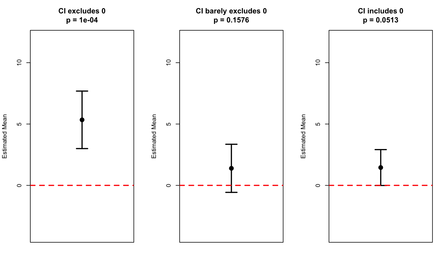
Always consider effect sizes alongside p-values. Report confidence intervals, which convey both the magnitude of an effect and the uncertainty about it. A 95% confidence interval that excludes zero is equivalent to statistical significance at $\alpha = 0.05$, but also shows the range of plausible effect sizes.

The Connection Between P-Values and Confidence Intervals

P-values and confidence intervals are mathematically linked. Understanding this connection deepens your grasp of both concepts.

For testing whether a parameter equals some null value $\theta_0$ (e.g., testing if $\mu = 0$ or $\mu_1 - \mu_2 = 0$):

The P-Value / CI Duality

If the $(1-\alpha)$ confidence interval excludes $\theta_0$, then $p < \alpha$
If the $(1-\alpha)$ confidence interval includes $\theta_0$, then $p \geq \alpha$

A 95% CI that doesn’t contain zero corresponds to p < 0.05 for a two-tailed test.

This relationship makes sense when you think about it: the confidence interval represents the range of parameter values that are “compatible” with the data. If the null value falls outside this range, the data provide evidence against it (small p-value). If the null value falls inside, the data are consistent with it (large p-value).

Code

# Demonstrate the CI-pvalue relationship
set.seed(42)

# Three scenarios
scenarios <- list(
  list(true_mean = 5, label = "CI excludes 0"),
  list(true_mean = 2, label = "CI barely excludes 0"),
  list(true_mean = 0.5, label = "CI includes 0")
)

par(mfrow = c(1, 3))

for (scenario in scenarios) {
  sample_data <- rnorm(30, mean = scenario$true_mean, sd = 5)
  result <- t.test(sample_data)

  # Plot CI
  ci <- result$conf.int
  mean_est <- result$estimate

  plot(1, mean_est, xlim = c(0.5, 1.5), ylim = c(-4, 12),
       pch = 19, cex = 1.5, xaxt = "n", xlab = "",
       ylab = "Estimated Mean",
       main = paste0(scenario$label, "\np = ", round(result$p.value, 4)))

  arrows(1, ci[1], 1, ci[2], angle = 90, code = 3, length = 0.1, lwd = 2)
  abline(h = 0, col = "red", lty = 2, lwd = 2)
}

Figure 16.7: The relationship between confidence intervals and p-values: CIs that exclude zero correspond to small p-values

The beauty of confidence intervals is that they provide more information than p-values alone:

Direction: You see whether the effect is positive or negative
Magnitude: You see the estimated size of the effect
Precision: The width shows your uncertainty
Significance: Whether zero is included tells you if p < 0.05

This is why many statisticians advocate for reporting confidence intervals as the primary summary, with p-values as secondary.

Standardized Effect Sizes

Effect sizes quantify the magnitude of an effect in a standardized way, allowing comparison across studies.

Cohen’s d measures the difference between two means in standard deviation units:

\[d = \frac{\bar{x}_1 - \bar{x}_2}{s_{\text{pooled}}}\]

where $s_{\text{pooled}} = \sqrt{\frac{(n_1-1)s_1^2 + (n_2-1)s_2^2}{n_1 + n_2 - 2}}$

Cohen’s guidelines suggest $d = 0.2$ is small, $d = 0.5$ is medium, and $d = 0.8$ is large, though these benchmarks should be interpreted in context (Cohen 1988).

Code

# Calculate Cohen's d
group1 <- c(23, 25, 28, 31, 27, 29)
group2 <- c(18, 20, 22, 19, 21, 23)

# Pooled standard deviation
n1 <- length(group1)
n2 <- length(group2)
s_pooled <- sqrt(((n1-1)*var(group1) + (n2-1)*var(group2)) / (n1 + n2 - 2))

# Cohen's d
cohens_d <- (mean(group1) - mean(group2)) / s_pooled
cat("Cohen's d:", round(cohens_d, 3), "\n")

Cohen's d: 2.76

Other effect sizes include: - Pearson’s r: Correlation coefficient (-1 to 1) - $\eta^2$ (eta-squared): Proportion of variance explained in ANOVA - Odds ratio: Effect size for binary outcomes

16.10 Critiques of NHST

The Null Hypothesis Significance Testing (NHST) framework, while widely used, has important limitations that researchers should understand.

Limitations of P-Values

P-values do not measure effect size: A tiny, meaningless effect can have p < 0.001 with enough data
P-values do not measure probability that $H_0$ is true: This is a common misinterpretation
The 0.05 threshold is arbitrary: There is nothing magical about $\alpha = 0.05$
Dichotomous thinking: Treating p = 0.049 and p = 0.051 as fundamentally different is misleading
Publication bias: Studies with p < 0.05 are more likely to be published, distorting the literature

Alternatives and Complements to NHST

Several approaches complement or provide alternatives to traditional null hypothesis significance testing. Confidence intervals offer richer information than p-values alone, communicating both the estimated effect size and the uncertainty surrounding it in a single, interpretable summary. Effect sizes quantify the practical magnitude of results in standardized units, allowing comparison across studies and helping distinguish statistical significance from practical importance. Bayesian methods reframe inference entirely, providing direct probability statements about hypotheses themselves rather than about the data conditional on a hypothesis. Finally, equivalence testing allows researchers to demonstrate that an effect is negligibly small—actively supporting the conclusion that groups are practically equivalent rather than merely failing to find a significant difference.

The American Statistical Association’s 2016 statement on p-values emphasizes that p-values should not be used in isolation and that scientific conclusions should not be based solely on whether a p-value crosses a threshold.

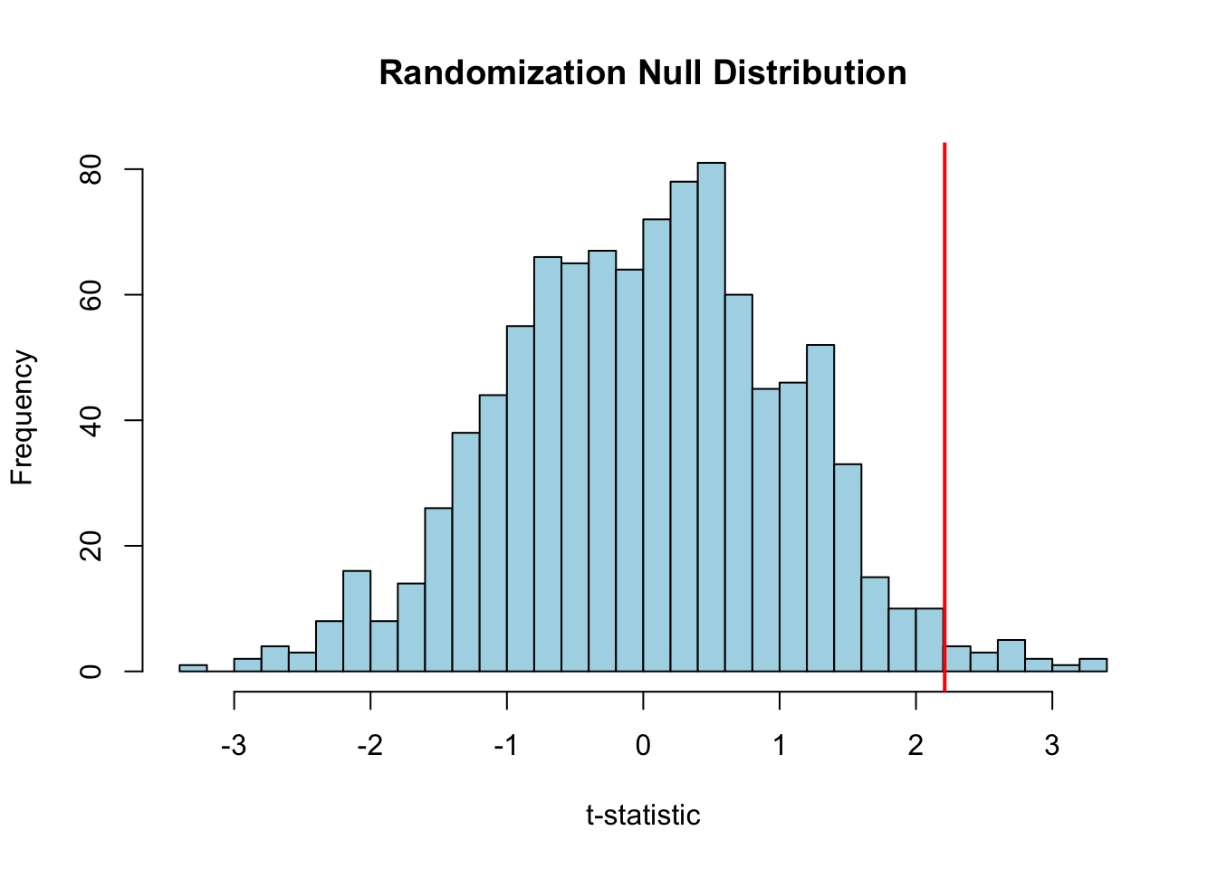
16.11 Example: Null Distribution via Randomization

We can create empirical null distributions through randomization, providing an alternative to parametric assumptions.

Code

# Two groups to compare
set.seed(56)
pop_1 <- rnorm(n = 50, mean = 20.1, sd = 2)
pop_2 <- rnorm(n = 50, mean = 19.3, sd = 2)

# Observed t-statistic
t_obs <- t.test(x = pop_1, y = pop_2, alternative = "greater")$statistic

# Create null distribution by randomization
pops_comb <- c(pop_1, pop_2)

t_rand <- replicate(1000, {
  pops_shuf <- sample(pops_comb)
  t.test(x = pops_shuf[1:50], y = pops_shuf[51:100], alternative = "greater")$statistic
})

# Plot null distribution
hist(t_rand, breaks = 30, main = "Randomization Null Distribution",
     xlab = "t-statistic", col = "lightblue")
abline(v = t_obs, col = "red", lwd = 2)

Figure 16.8: Randomization creates an empirical null distribution; the red line shows the observed test statistic

Code

# Calculate p-value
p_value <- sum(t_rand >= t_obs) / 1000
cat("Observed t:", round(t_obs, 3), "\n")

Observed t: 2.211

Code

cat("P-value:", p_value, "\n")

P-value: 0.016

Figure 16.9: Randomization tests provide a distribution-free alternative to parametric tests

16.12 Summary

Hypothesis testing provides a framework for using data to evaluate claims about populations. Key concepts include:

Null and alternative hypotheses formalize competing claims
Type I errors (false positives) and Type II errors (false negatives) represent the two ways we can be wrong
P-values quantify evidence against the null hypothesis
Significance levels set thresholds for decision-making
Multiple testing requires adjustment to control error rates
Statistical significance does not imply practical importance

In the following chapters, we apply this framework to specific tests: t-tests for comparing means, chi-squared tests for categorical data, and nonparametric alternatives when assumptions are violated.

16.13 Exercises

Exercise H.1: Understanding Type I and Type II Errors

Consider a diagnostic test for a rare disease that affects 1% of the population. The test has a false positive rate (Type I error) of 5% and a false negative rate (Type II error) of 10%.

Define the null and alternative hypotheses for this diagnostic test
What does a Type I error mean in this context? What are the consequences?
What does a Type II error mean in this context? What are the consequences?
If 10,000 people are tested, how many false positives and false negatives would you expect?
Of the people who test positive, what proportion actually have the disease? (This is related to the positive predictive value)

Code

# Your code here

Exercise H.2: P-Values and Interpretation

For each statement below, indicate whether it is a correct interpretation of p = 0.03:

The probability that the null hypothesis is true is 0.03
The probability of observing data this extreme or more extreme, given that the null hypothesis is true, is 0.03
The probability that the result occurred by chance is 0.03
There is a 97% probability that the alternative hypothesis is true
If we repeated this experiment many times, we would expect to see results this extreme about 3% of the time if the null hypothesis were true

For the correct interpretation(s), explain why they are correct. For the incorrect ones, explain the mistake.

Exercise H.3: Power Analysis

You are planning a study to compare the effectiveness of two fertilizers on plant growth. Based on pilot data, you estimate the standard deviation of plant heights to be 12 cm. You want to detect a difference of 8 cm between treatments with 80% power at α = 0.05.

Calculate the required sample size per group using the pwr.t.test() function
Create a power curve showing how power changes with sample size for this effect size
How much would the required sample size change if you wanted 90% power instead of 80%?
If your budget only allows for 20 plants per group, what is the smallest effect size (in Cohen’s d units) you could detect with 80% power?
Discuss the trade-offs between sample size, power, and minimum detectable effect size

Code

# Your code here
library(pwr)

Exercise H.4: Multiple Testing Correction

A genomics study tests 20,000 genes for differential expression between two conditions, using α = 0.05 for each test.

If all null hypotheses are true (no genes are differentially expressed), how many false positives (Type I errors) would you expect on average?
Apply the Bonferroni correction. What significance threshold should be used for each individual test?
Why might the Bonferroni correction be too conservative in this context?
Simulate a scenario where 100 genes are truly differentially expressed (with effect size d = 0.8, n = 10 per group) and 19,900 are not. How many true positives and false positives do you get with:
- No correction (α = 0.05)
- Bonferroni correction
- Use the p.adjust() function with method “fdr” for False Discovery Rate control

Code

# Your code here

Exercise H.5: Confidence Intervals vs. P-Values

You conduct an experiment measuring the effect of a drug on blood glucose levels. You measure 15 patients before and after treatment and find: - Mean difference: -12.3 mg/dL - 95% CI: [-22.1, -2.5] - p-value: 0.018

Based on the confidence interval alone, what can you conclude about the null hypothesis that the drug has no effect?
Explain the relationship between the confidence interval and the p-value in this example
If you calculated a 99% confidence interval instead, would it include zero? Would the p-value be less than 0.01? Explain your reasoning.
Generate simulated data consistent with these results and verify the relationship between the CI and p-value

Code

# Your code here

Exercise H.6: Randomization Test

You have two groups of seedlings grown under different light conditions:

group_A <- c(12.3, 14.1, 13.5, 15.2, 13.8, 14.9, 13.2, 14.5)
group_B <- c(10.8, 11.5, 12.1, 11.2, 10.9, 12.4, 11.8, 11.3)

Calculate the observed difference in means (group A - group B)
Perform a randomization test with 10,000 permutations to generate a null distribution
Calculate the p-value from your randomization test
Compare this to the p-value from a two-sample t-test
Create a histogram of the null distribution with a vertical line showing the observed difference
Under what circumstances might the randomization test be preferable to the t-test?

Code

# Your code here

16.14 Additional Resources

Cohen (1988) - The classic reference on statistical power analysis
Logan (2010) - Comprehensive treatment of hypothesis testing in biological contexts

# Hypothesis Testing {#sec-hypothesis-testing} ```{r} #| echo: false #| message: false library(tidyverse) theme_set(theme_minimal()) ``` ## What is a Hypothesis? A hypothesis is a statement of belief about the world—a claim that can be evaluated with data. In statistics, we formalize hypothesis testing as a framework for using data to decide between competing claims. The **null hypothesis** ($H_0$) represents a default position, typically stating that there is no effect, no difference, or no relationship. The **alternative hypothesis** ($H_A$) represents what we would conclude if we reject the null—typically that there is an effect, difference, or relationship. For example, consider testing whether an amino acid substitution changes the catalytic rate of an enzyme: - $H_0$: The substitution does not change the catalytic rate - $H_A$: The substitution does change the catalytic rate The alternative hypothesis might be directional (the substitution increases the rate) or non-directional (the substitution changes the rate, in either direction). This distinction affects how we calculate p-values. ## The Logic of Hypothesis Testing Hypothesis testing follows a specific logic. We assume the null hypothesis is true and ask: how likely would we be to observe data as extreme as what we actually observed? If this probability is very small, we conclude that the null hypothesis is unlikely to be true and reject it in favor of the alternative. This framework naturally raises several key questions. What is the probability that we might reject a true null hypothesis, committing a false positive error? Conversely, what is the probability that we might fail to reject a false null hypothesis, missing a real effect? How do we decide when the evidence is strong enough to reject the null hypothesis? And perhaps most subtly, what can we legitimately conclude when we fail to reject the null—does this mean we've proven it true, or merely that we lack sufficient evidence against it? ## Type I and Type II Errors Two types of mistakes are possible in hypothesis testing.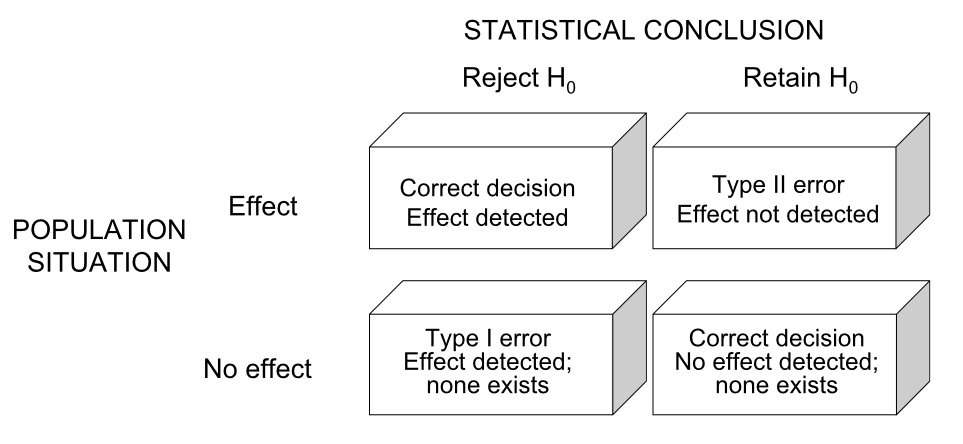 ![Type I and Type II errors in hypothesis testing](../images/ch15/ch15_error_types.jpeg){#fig-error-types fig-align="center"} A **Type I error** occurs when we reject a true null hypothesis—concluding there is an effect when there is not. The probability of a Type I error is denoted $\alpha$ and is called the significance level. By convention, $\alpha$ is often set to 0.05, meaning we accept a 5% chance of falsely rejecting a true null.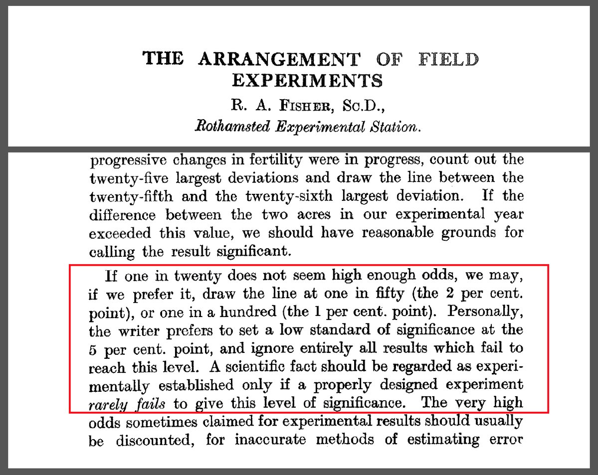 ![R.A. Fisher's original 1926 paper "The Arrangement of Field Experiments" where he proposed the 0.05 significance threshold. Fisher wrote that results reaching "the 5 per cent. point" provide "reasonable grounds for calling the result significant." This arbitrary but practical convention has shaped statistical practice for nearly a century.](../images/ch15/ch15_fisher_pvalue.jpg){#fig-fisher-pvalue fig-align="center" width="80%"} A **Type II error** occurs when we fail to reject a false null hypothesis—concluding there is no effect when there actually is one. The probability of a Type II error is denoted $\beta$. **Power** is the probability of correctly rejecting a false null hypothesis: Power = $1 - \beta$. Power depends on the effect size (how big the true effect is), sample size, significance level, and variability in the data. | | $H_0$ True | $H_0$ False | |:--|:--|:--| | Reject $H_0$ | Type I Error ($\alpha$) | Correct Decision (Power) | | Fail to Reject $H_0$ | Correct Decision | Type II Error ($\beta$) | ### Understanding Statistical Power Power analysis is essential for designing experiments that can actually detect effects of interest. A study with low power is unlikely to find real effects even when they exist—wasting resources and potentially leading to incorrect conclusions. Several key factors determine statistical power. **Effect size** matters fundamentally—larger effects are easier to detect than subtle ones. **Sample size** directly affects power because more data provides more information about the true state of nature. The chosen **significance level ($\alpha$)** creates a trade-off: higher $\alpha$ increases power to detect true effects but also increases the Type I error rate. Finally, **variability** in the data affects how clearly we can see signals; less noise makes true effects easier to detect, while high variability obscures even substantial effects. For a two-sample t-test, the relationship between these factors can be expressed approximately as: $$\text{Power} \approx \Phi\left(\frac{|\mu_1 - \mu_2|}{\sigma}\sqrt{\frac{n}{2}} - z_{1-\alpha/2}\right)$$ where $\Phi$ is the standard normal CDF, and $z_{1-\alpha/2}$ is the critical value. ```{r} #| label: fig-power-curves #| fig-cap: "Statistical power increases with sample size and effect size; the dashed line indicates the common 80% power threshold" #| fig-width: 8 #| fig-height: 5 # Visualize how power depends on effect size and sample size library(pwr) # Power curves for different effect sizes effect_sizes <- c(0.2, 0.5, 0.8) # Cohen's d: small, medium, large sample_sizes <- seq(5, 100, by = 5) par(mfrow = c(1, 1)) colors <- c("blue", "darkgreen", "red") plot(NULL, xlim = c(5, 100), ylim = c(0, 1), xlab = "Sample Size (per group)", ylab = "Power", main = "Power Curves for Two-Sample t-Test") abline(h = 0.8, lty = 2, col = "gray") for (i in 1:3) { powers <- sapply(sample_sizes, function(n) { pwr.t.test(n = n, d = effect_sizes[i], sig.level = 0.05, type = "two.sample")$power }) lines(sample_sizes, powers, col = colors[i], lwd = 2) } legend("bottomright", legend = c("Small (d=0.2)", "Medium (d=0.5)", "Large (d=0.8)"), col = colors, lwd = 2) ``` ### A Priori Power Analysis Before conducting an experiment, power analysis helps determine the necessary sample size. The question is: "How many observations do I need to have an 80% chance of detecting an effect of a given size?" ```{r} # Sample size calculation for 80% power # Detecting a medium effect (d = 0.5) with alpha = 0.05 power_result <- pwr.t.test(d = 0.5, sig.level = 0.05, power = 0.8, type = "two.sample") cat("Required sample size per group:", ceiling(power_result$n), "\n") # For a small effect (d = 0.2) power_small <- pwr.t.test(d = 0.2, sig.level = 0.05, power = 0.8, type = "two.sample") cat("For small effect (d=0.2):", ceiling(power_small$n), "per group\n") ``` Notice how detecting small effects requires substantially larger samples. This is why pilot studies and literature-based effect size estimates are valuable for planning. ## P-Values The **p-value** is the probability of observing a test statistic as extreme or more extreme than the one calculated from the data, assuming the null hypothesis is true. A small p-value indicates that the observed data would be unlikely if the null hypothesis were true, providing evidence against the null. A large p-value indicates that the data are consistent with the null hypothesis. The p-value is NOT the probability that the null hypothesis is true. It is the probability of the data (or more extreme data) given the null hypothesis, not the probability of the null hypothesis given the data. ## Significance Level and Decision Rules The **significance level** $\alpha$ is the threshold below which we reject the null hypothesis. If $p < \alpha$, we reject $H_0$. If $p \geq \alpha$, we fail to reject $H_0$.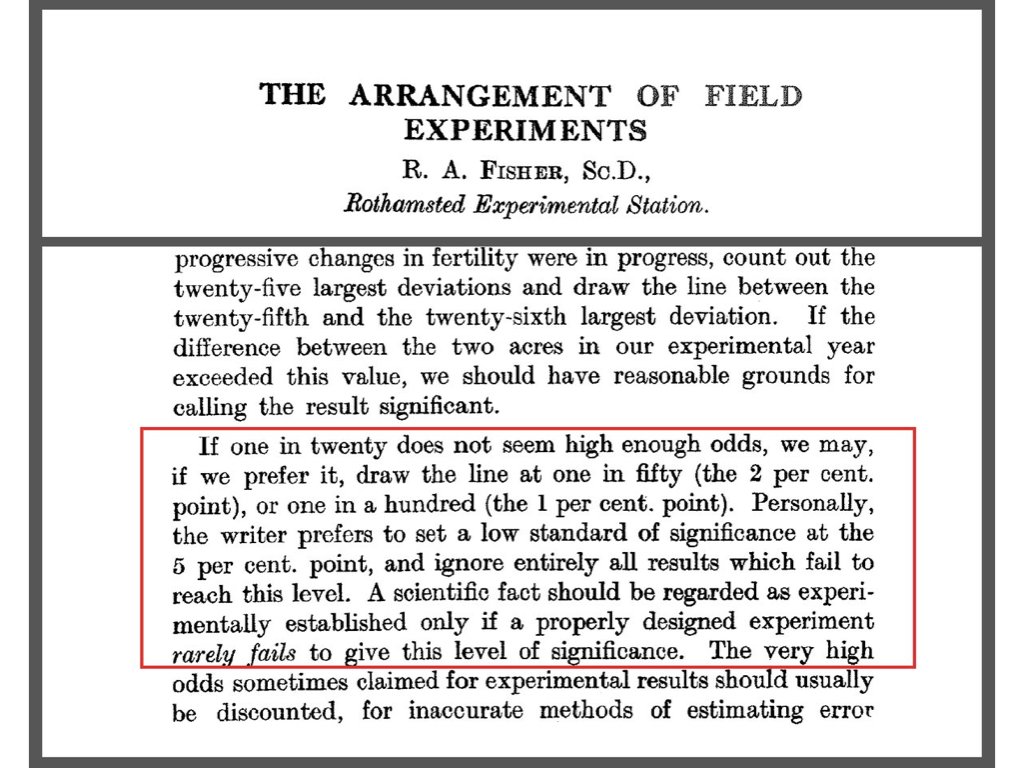 ![The significance level α determines the rejection region for hypothesis testing](../images/ch15/ch15_significance_level.jpeg){#fig-significance-level fig-align="center"} The conventional choice of $\alpha = 0.05$ is arbitrary but widely used. In contexts where Type I errors are particularly costly (e.g., approving an ineffective drug), smaller $\alpha$ values may be appropriate. In exploratory research, larger $\alpha$ values might be acceptable. Important: "fail to reject" is not the same as "accept." Failing to reject the null hypothesis means the data did not provide sufficient evidence against it, not that the null hypothesis is true. ## Test Statistics and Statistical Distributions A **test statistic** summarizes the data in a way that allows comparison to a known distribution under the null hypothesis. Different tests use different statistics: the t-statistic for t-tests, the F-statistic for ANOVA, the chi-squared statistic for contingency tables. Just like raw data, test statistics are random variables with their own sampling distributions. Under the null hypothesis, we know what distribution the test statistic should follow. We can then calculate how unusual our observed statistic is under this distribution.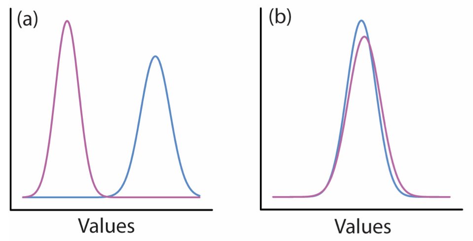 ![Test statistics follow known distributions under the null hypothesis](../images/ch15/ch15_test_statistic.jpeg){#fig-test-statistic fig-align="center"} ## One-Tailed vs. Two-Tailed Tests A **two-tailed test** considers extreme values in both directions. The alternative hypothesis is non-directional: $H_A: \mu \neq \mu_0$. Extreme values in either tail of the distribution count as evidence against the null. A **one-tailed test** considers extreme values in only one direction. The alternative hypothesis is directional: $H_A: \mu > \mu_0$ or $H_A: \mu < \mu_0$. Only extreme values in the specified direction count as evidence against the null.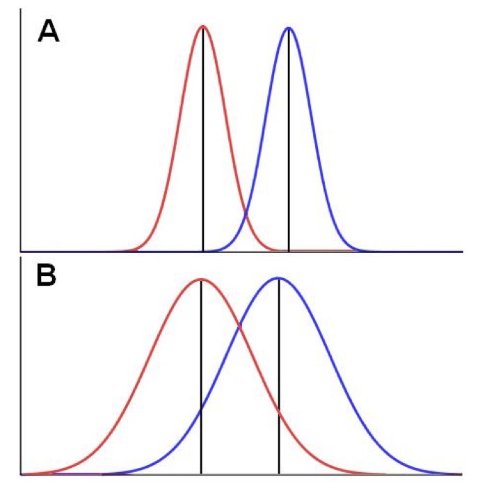 ![One-tailed vs. two-tailed tests: the alternative hypothesis determines which tail(s) to consider](../images/ch15/ch15_tailed_tests.jpeg){#fig-tailed-tests fig-align="center"} Two-tailed tests are more conservative and are appropriate when you do not have a strong prior expectation about the direction of an effect. One-tailed tests have more power to detect effects in the specified direction but will miss effects in the opposite direction. ## Multiple Testing When you perform many hypothesis tests, the probability of at least one Type I error increases. If you test 20 independent hypotheses at $\alpha = 0.05$, you expect about one false positive even when all null hypotheses are true. Several approaches address multiple testing: **Bonferroni correction** divides $\alpha$ by the number of tests. For 20 tests, use $\alpha = 0.05/20 = 0.0025$. This is conservative and may miss true effects. **False Discovery Rate (FDR)** control allows some false positives but controls their proportion among rejected hypotheses. This is less conservative than Bonferroni and widely used in genomics and other high-throughput applications. ## Practical vs. Statistical Significance Statistical significance does not imply practical importance. With a large enough sample, even trivially small effects become statistically significant. Conversely, practically important effects may not reach statistical significance with small samples. Always consider effect sizes alongside p-values. Report confidence intervals, which convey both the magnitude of an effect and the uncertainty about it. A 95% confidence interval that excludes zero is equivalent to statistical significance at $\alpha = 0.05$, but also shows the range of plausible effect sizes. ### The Connection Between P-Values and Confidence Intervals P-values and confidence intervals are mathematically linked. Understanding this connection deepens your grasp of both concepts. For testing whether a parameter equals some null value $\theta_0$ (e.g., testing if $\mu = 0$ or $\mu_1 - \mu_2 = 0$): ::: {.callout-tip} ## The P-Value / CI Duality - If the $(1-\alpha)$ confidence interval **excludes** $\theta_0$, then $p < \alpha$ - If the $(1-\alpha)$ confidence interval **includes** $\theta_0$, then $p \geq \alpha$ A 95% CI that doesn't contain zero corresponds to p < 0.05 for a two-tailed test. ::: This relationship makes sense when you think about it: the confidence interval represents the range of parameter values that are "compatible" with the data. If the null value falls outside this range, the data provide evidence against it (small p-value). If the null value falls inside, the data are consistent with it (large p-value). ```{r} #| label: fig-ci-pvalue-relationship #| fig-cap: "The relationship between confidence intervals and p-values: CIs that exclude zero correspond to small p-values" #| fig-width: 8 #| fig-height: 5 # Demonstrate the CI-pvalue relationship set.seed(42) # Three scenarios scenarios <- list( list(true_mean = 5, label = "CI excludes 0"), list(true_mean = 2, label = "CI barely excludes 0"), list(true_mean = 0.5, label = "CI includes 0") ) par(mfrow = c(1, 3)) for (scenario in scenarios) { sample_data <- rnorm(30, mean = scenario$true_mean, sd = 5) result <- t.test(sample_data) # Plot CI ci <- result$conf.int mean_est <- result$estimate plot(1, mean_est, xlim = c(0.5, 1.5), ylim = c(-4, 12), pch = 19, cex = 1.5, xaxt = "n", xlab = "", ylab = "Estimated Mean", main = paste0(scenario$label, "\np = ", round(result$p.value, 4))) arrows(1, ci[1], 1, ci[2], angle = 90, code = 3, length = 0.1, lwd = 2) abline(h = 0, col = "red", lty = 2, lwd = 2) } ``` The beauty of confidence intervals is that they provide *more* information than p-values alone: 1. **Direction**: You see whether the effect is positive or negative 2. **Magnitude**: You see the estimated size of the effect 3. **Precision**: The width shows your uncertainty 4. **Significance**: Whether zero is included tells you if p < 0.05 This is why many statisticians advocate for reporting confidence intervals as the primary summary, with p-values as secondary. ### Standardized Effect Sizes Effect sizes quantify the magnitude of an effect in a standardized way, allowing comparison across studies. **Cohen's d** measures the difference between two means in standard deviation units: $$d = \frac{\bar{x}_1 - \bar{x}_2}{s_{\text{pooled}}}$$ where $s_{\text{pooled}} = \sqrt{\frac{(n_1-1)s_1^2 + (n_2-1)s_2^2}{n_1 + n_2 - 2}}$ Cohen's guidelines suggest $d = 0.2$ is small, $d = 0.5$ is medium, and $d = 0.8$ is large, though these benchmarks should be interpreted in context [@cohen1988statistical]. ```{r} # Calculate Cohen's d group1 <- c(23, 25, 28, 31, 27, 29) group2 <- c(18, 20, 22, 19, 21, 23) # Pooled standard deviation n1 <- length(group1) n2 <- length(group2) s_pooled <- sqrt(((n1-1)*var(group1) + (n2-1)*var(group2)) / (n1 + n2 - 2)) # Cohen's d cohens_d <- (mean(group1) - mean(group2)) / s_pooled cat("Cohen's d:", round(cohens_d, 3), "\n") ``` Other effect sizes include: - **Pearson's r**: Correlation coefficient (-1 to 1) - **$\eta^2$ (eta-squared)**: Proportion of variance explained in ANOVA - **Odds ratio**: Effect size for binary outcomes ## Critiques of NHST The Null Hypothesis Significance Testing (NHST) framework, while widely used, has important limitations that researchers should understand. ::: {.callout-warning} ## Limitations of P-Values 1. **P-values do not measure effect size**: A tiny, meaningless effect can have p < 0.001 with enough data 2. **P-values do not measure probability that $H_0$ is true**: This is a common misinterpretation 3. **The 0.05 threshold is arbitrary**: There is nothing magical about $\alpha = 0.05$ 4. **Dichotomous thinking**: Treating p = 0.049 and p = 0.051 as fundamentally different is misleading 5. **Publication bias**: Studies with p < 0.05 are more likely to be published, distorting the literature ::: ### Alternatives and Complements to NHST Several approaches complement or provide alternatives to traditional null hypothesis significance testing. **Confidence intervals** offer richer information than p-values alone, communicating both the estimated effect size and the uncertainty surrounding it in a single, interpretable summary. **Effect sizes** quantify the practical magnitude of results in standardized units, allowing comparison across studies and helping distinguish statistical significance from practical importance. **Bayesian methods** reframe inference entirely, providing direct probability statements about hypotheses themselves rather than about the data conditional on a hypothesis. Finally, **equivalence testing** allows researchers to demonstrate that an effect is negligibly small—actively supporting the conclusion that groups are practically equivalent rather than merely failing to find a significant difference. The American Statistical Association's 2016 statement on p-values emphasizes that p-values should not be used in isolation and that scientific conclusions should not be based solely on whether a p-value crosses a threshold. ## Example: Null Distribution via Randomization We can create empirical null distributions through randomization, providing an alternative to parametric assumptions. ```{r} #| label: fig-randomization-null #| fig-cap: "Randomization creates an empirical null distribution; the red line shows the observed test statistic" #| fig-width: 7 #| fig-height: 5 # Two groups to compare set.seed(56) pop_1 <- rnorm(n = 50, mean = 20.1, sd = 2) pop_2 <- rnorm(n = 50, mean = 19.3, sd = 2) # Observed t-statistic t_obs <- t.test(x = pop_1, y = pop_2, alternative = "greater")$statistic # Create null distribution by randomization pops_comb <- c(pop_1, pop_2) t_rand <- replicate(1000, { pops_shuf <- sample(pops_comb) t.test(x = pops_shuf[1:50], y = pops_shuf[51:100], alternative = "greater")$statistic }) # Plot null distribution hist(t_rand, breaks = 30, main = "Randomization Null Distribution", xlab = "t-statistic", col = "lightblue") abline(v = t_obs, col = "red", lwd = 2) ``` ```{r} # Calculate p-value p_value <- sum(t_rand >= t_obs) / 1000 cat("Observed t:", round(t_obs, 3), "\n") cat("P-value:", p_value, "\n")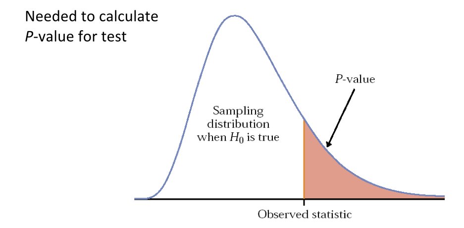 ``` ![Randomization tests provide a distribution-free alternative to parametric tests](../images/ch15/ch15_randomization.jpeg){#fig-randomization-concept fig-align="center"} ## Summary Hypothesis testing provides a framework for using data to evaluate claims about populations. Key concepts include: - Null and alternative hypotheses formalize competing claims - Type I errors (false positives) and Type II errors (false negatives) represent the two ways we can be wrong - P-values quantify evidence against the null hypothesis - Significance levels set thresholds for decision-making - Multiple testing requires adjustment to control error rates - Statistical significance does not imply practical importance In the following chapters, we apply this framework to specific tests: t-tests for comparing means, chi-squared tests for categorical data, and nonparametric alternatives when assumptions are violated. ## Exercises ::: {.callout-note} ### Exercise H.1: Understanding Type I and Type II Errors Consider a diagnostic test for a rare disease that affects 1% of the population. The test has a false positive rate (Type I error) of 5% and a false negative rate (Type II error) of 10%. a) Define the null and alternative hypotheses for this diagnostic test b) What does a Type I error mean in this context? What are the consequences? c) What does a Type II error mean in this context? What are the consequences? d) If 10,000 people are tested, how many false positives and false negatives would you expect? e) Of the people who test positive, what proportion actually have the disease? (This is related to the positive predictive value) ```{r} #| eval: false # Your code here ``` ::: ::: {.callout-note} ### Exercise H.2: P-Values and Interpretation For each statement below, indicate whether it is a correct interpretation of p = 0.03: a) The probability that the null hypothesis is true is 0.03 b) The probability of observing data this extreme or more extreme, given that the null hypothesis is true, is 0.03 c) The probability that the result occurred by chance is 0.03 d) There is a 97% probability that the alternative hypothesis is true e) If we repeated this experiment many times, we would expect to see results this extreme about 3% of the time if the null hypothesis were true For the correct interpretation(s), explain why they are correct. For the incorrect ones, explain the mistake. ::: ::: {.callout-note} ### Exercise H.3: Power Analysis You are planning a study to compare the effectiveness of two fertilizers on plant growth. Based on pilot data, you estimate the standard deviation of plant heights to be 12 cm. You want to detect a difference of 8 cm between treatments with 80% power at α = 0.05. a) Calculate the required sample size per group using the `pwr.t.test()` function b) Create a power curve showing how power changes with sample size for this effect size c) How much would the required sample size change if you wanted 90% power instead of 80%? d) If your budget only allows for 20 plants per group, what is the smallest effect size (in Cohen's d units) you could detect with 80% power? e) Discuss the trade-offs between sample size, power, and minimum detectable effect size ```{r} #| eval: false # Your code here library(pwr) ``` ::: ::: {.callout-note} ### Exercise H.4: Multiple Testing Correction A genomics study tests 20,000 genes for differential expression between two conditions, using α = 0.05 for each test. a) If all null hypotheses are true (no genes are differentially expressed), how many false positives (Type I errors) would you expect on average? b) Apply the Bonferroni correction. What significance threshold should be used for each individual test? c) Why might the Bonferroni correction be too conservative in this context? d) Simulate a scenario where 100 genes are truly differentially expressed (with effect size d = 0.8, n = 10 per group) and 19,900 are not. How many true positives and false positives do you get with: - No correction (α = 0.05) - Bonferroni correction - Use the `p.adjust()` function with method "fdr" for False Discovery Rate control ```{r} #| eval: false # Your code here ``` ::: ::: {.callout-note} ### Exercise H.5: Confidence Intervals vs. P-Values You conduct an experiment measuring the effect of a drug on blood glucose levels. You measure 15 patients before and after treatment and find: - Mean difference: -12.3 mg/dL - 95% CI: [-22.1, -2.5] - p-value: 0.018 a) Based on the confidence interval alone, what can you conclude about the null hypothesis that the drug has no effect? b) Explain the relationship between the confidence interval and the p-value in this example c) If you calculated a 99% confidence interval instead, would it include zero? Would the p-value be less than 0.01? Explain your reasoning. d) Generate simulated data consistent with these results and verify the relationship between the CI and p-value ```{r} #| eval: false # Your code here ``` ::: ::: {.callout-note} ### Exercise H.6: Randomization Test You have two groups of seedlings grown under different light conditions: ``` group_A <- c(12.3, 14.1, 13.5, 15.2, 13.8, 14.9, 13.2, 14.5) group_B <- c(10.8, 11.5, 12.1, 11.2, 10.9, 12.4, 11.8, 11.3) ``` a) Calculate the observed difference in means (group A - group B) b) Perform a randomization test with 10,000 permutations to generate a null distribution c) Calculate the p-value from your randomization test d) Compare this to the p-value from a two-sample t-test e) Create a histogram of the null distribution with a vertical line showing the observed difference f) Under what circumstances might the randomization test be preferable to the t-test? ```{r} #| eval: false # Your code here ``` ::: ## Additional Resources - @cohen1988statistical - The classic reference on statistical power analysis - @logan2010biostatistical - Comprehensive treatment of hypothesis testing in biological contexts

	\(H_0\) True	\(H_0\) False
Reject \(H_0\)	Type I Error (\(\alpha\))	Correct Decision (Power)
Fail to Reject \(H_0\)	Correct Decision	Type II Error (\(\beta\))