Figure 7.1: Tidy data principles provide a standard way to organize datasets
7.1 What is Tidy Data?
Data comes in many shapes, and not all shapes are equally convenient for analysis. The concept of “tidy data” provides a standard way to organize data that works well with R and makes many analyses straightforward. In tidy data, each variable forms a column, each observation forms a row, and each type of observational unit forms a table.
Figure 7.2: In tidy data, each variable forms a column and each observation forms a row
This structure might seem obvious, but real-world data rarely arrives in tidy form. Spreadsheets often encode information in column names, spread a single variable across multiple columns, or combine multiple variables in a single column. Data wrangling is the process of transforming messy data into tidy data.
The three interrelated rules that make a dataset tidy are:
Each variable forms a column
Each observation forms a row
Each type of observational unit forms a table
These rules are interrelated because it is impossible to satisfy only two of the three. This interrelationship leads to an even simpler set of practical instructions:
Put each dataset in a tibble (or data frame)
Put each variable in a column
7.2 Types of Data
Understanding the types of data you are working with guides how you analyze them and how they should be represented in R.
Categorical Data
Categorical data classify observations into groups. There are two main types:
Nominal categorical data have no inherent order. Examples include: - Species names (e.g., Homo sapiens, Mus musculus) - Treatment groups (control, treatment A, treatment B) - Colors (red, blue, green) - Gene names (BRCA1, TP53, EGFR)
Ordinal categorical data have a meaningful order, but the distances between categories may not be equal. Examples include: - Ratings (low, medium, high) - Educational levels (high school, bachelor’s, master’s, doctorate) - Disease severity (mild, moderate, severe) - T-shirt sizes (small, medium, large, extra large)
In R, categorical data are typically represented as factors, which store both the values and the set of possible levels. Factors are essential for statistical modeling and ensure that categories are handled consistently.
Quantitative Data
Quantitative data are numerical measurements. Understanding the scale of measurement is important for choosing appropriate statistical tests.
Discrete quantitative data can only take specific values, usually whole numbers: - Counts (number of offspring, number of cells) - Integers (age in years) - Scores on a fixed scale
Continuous quantitative data can theoretically take any value within a range: - Mass, length, volume - Temperature - Concentration - Gene expression levels
Quantitative data can also be classified by their scale properties:
Interval data have meaningful differences between values but no true zero point: - Temperature in Celsius or Fahrenheit (0° does not mean “no temperature”) - Calendar dates (year 0 is arbitrary) - pH scale
Ratio data have a true zero and meaningful ratios: - Mass, length, volume (zero means “none”) - Counts (zero means “zero items”) - Concentration (zero means “nothing present”) - Time duration
The distinction matters because ratio data support statements like “twice as much” while interval data do not. Water at 20°C is not “twice as hot” as water at 10°C, but 20 grams is twice as heavy as 10 grams.
Data Types in R
Different types of data are represented by different data types in R. Understanding these types helps you work with data more effectively.
Data Type
Description
Examples
R Type
Character
Text strings
“control”, “treatment”, gene names
character
Factor
Categorical with levels, unordered
Species, treatment groups, colors
factor
Ordered Factor
Categorical with meaningful order
“low” < “medium” < “high”
ordered
Integer
Whole numbers
Count data, discrete measurements
integer
Numeric
Real numbers (decimal)
Measurements, ratios, continuous data
numeric or double
Logical
True/false values
Test results, conditions
logical
Date
Calendar dates
“2024-01-15”, sample collection dates
Date
Date-Time
Timestamps with time
“2024-01-15 14:30:00”
POSIXct
You can check the type of any variable using the class() or typeof() functions:
Code
# Examples of different data typesx <-"hello"# charactery <-factor(c("A", "B", "A")) # factorz <-42# numericw <-42L # integer (the L suffix)v <-TRUE# logicald <-as.Date("2024-01-15") # Date# Check typesclass(x)
[1] "character"
Code
class(y)
[1] "factor"
Code
class(z)
[1] "numeric"
Code
typeof(z)
[1] "double"
Code
class(w)
[1] "integer"
Code
typeof(w)
[1] "integer"
Code
class(v)
[1] "logical"
Code
class(d)
[1] "Date"
Understanding these types is crucial because:
Statistical functions expect specific data types
Categorical variables should be factors for modeling
Plotting functions treat factors differently from character strings
Mathematical operations only work on numeric types
7.3 Data File Best Practices
When working with data files, following consistent practices will save you time and prevent errors. These guidelines apply whether you are using Unix tools, R, or any other analysis software.
Do
Store data in plain text formats such as tab-separated (.tsv) or comma-separated (.csv) files. These nonproprietary formats can be read by any software and will remain accessible for years to come.
Keep an unedited copy of original data files. Even when your analysis requires modifications, preserve the raw data separately.
Use descriptive, consistent names for files and variables. A name like experiment1_control_measurements.tsv is far more useful than data2.txt.
Maintain metadata that documents what each variable means, how data were collected, and any processing steps applied.
Add new observations as rows and new variables as columns to maintain a consistent rectangular structure.
Include a header row with variable names that are concise but descriptive.
Use consistent date formats, preferably ISO 8601 format (YYYY-MM-DD).
Represent missing values consistently, typically as empty cells or NA.
Don’t
Don’t mix data types within a column. If a column contains numbers, every entry should be a number (or explicitly missing).
Don’t use special characters in file or directory names. Stick to letters, numbers, underscores, and hyphens. Avoid spaces, which can cause problems with command-line tools.
Don’t use delimiter characters in data values. If your file is comma-delimited, don’t use commas within data entries. For example, use 2024-03-08 rather than March 8, 2024 for dates.
Don’t copy data from formatted documents like Microsoft Word directly into data files. Hidden formatting characters can corrupt your data.
Don’t edit data files in spreadsheet programs that might silently convert values (for example, Excel’s tendency to convert gene names like SEPT1 to dates).
Don’t use color or formatting to encode information. All information should be in the cell values themselves, not in formatting that will be lost.
Don’t leave empty rows or columns as visual separators. These can cause problems when reading data into analysis software.
Preserving Raw Data
Perhaps the most important principle is to never modify your original raw data files. Keep them in a separate directory with restricted write permissions if possible. All data cleaning and transformation should be done programmatically (in scripts that can be re-run), with outputs saved to new files.
7.4 The Tidyverse
The tidyverse is a collection of R packages designed for data science. These packages share a common philosophy and are designed to work together seamlessly. The core tidyverse packages include:
ggplot2: Data visualization using the grammar of graphics
dplyr: Data manipulation and transformation
tidyr: Reshaping and tidying data
readr: Reading rectangular data (CSV, TSV, etc.)
purrr: Functional programming tools
tibble: Enhanced data frames
stringr: String manipulation
forcats: Working with factors (categorical data)
Figure 7.3: The tidyverse is a collection of R packages designed for data science
Loading the tidyverse loads all core packages at once:
Code
library(tidyverse)
The message shows which packages are attached and notes any functions that conflict with base R or other packages. For example, dplyr::filter() masks stats::filter(), meaning if you type filter(), you will get the dplyr version. To use the stats version, you would need to specify stats::filter() explicitly.
7.5 Tibbles
Tibbles are the tidyverse’s enhanced data frames. They are designed to be more user-friendly and consistent than traditional data frames, while maintaining backward compatibility for most operations.
Figure 7.4: Tibbles are the tidyverse’s enhanced data frames with improved printing
Creating Tibbles
You can create tibbles using the tibble() function:
# A tibble: 4 × 4
  name    age height_cm treatment
  <chr> <dbl>     <dbl> <fct>
1 Alice    25       165 control
2 Bob      32       178 drug_A
3 Carol    28       172 drug_A
4 David    45       180 control
You can also convert existing data frames to tibbles:
Code
# Convert a data frame to a tibbleiris_tibble <-as_tibble(iris)iris_tibble
Better printing: Tibbles print more informatively than data frames. They show: - Only the first 10 rows by default - Only columns that fit on screen - The dimensions (rows × columns) - The data type of each column (shown below the column name)
The column type abbreviations include: - <chr>: character strings - <dbl>: double (numeric with decimals) - <int>: integer - <lgl>: logical (TRUE/FALSE) - <fct>: factor - <date>: dates
Stricter subsetting: Tibbles never do partial matching of names and always generate a warning if you try to access a column that doesn’t exist.
No row names: Tibbles don’t use row names (they are never useful). If you have meaningful row names, convert them to a proper column.
Consistent subsetting: [ always returns a tibble, and $ doesn’t do partial matching.
Working with Tibbles
Most functions that work with data frames also work with tibbles:
Code
# Dimensionsdim(my_tibble)
[1] 4 4
Code
nrow(my_tibble)
[1] 4
Code
ncol(my_tibble)
[1] 4
Code
# Column namesnames(my_tibble)
[1] "name" "age" "height_cm" "treatment"
Code
colnames(my_tibble)
[1] "name" "age" "height_cm" "treatment"
Code
# Summary statisticssummary(my_tibble)
     name                age          height_cm       treatment
 Length:4           Min.   :25.00   Min.   :165.0   control:2
 Class :character   1st Qu.:27.25   1st Qu.:170.2   drug_A :2
 Mode  :character   Median :30.00   Median :175.0
                    Mean   :32.50   Mean   :173.8
                    3rd Qu.:35.25   3rd Qu.:178.5
                    Max.   :45.00   Max.   :180.0
You can extract columns as vectors using $ or [[:
Code
# Extract the 'name' column as a vectormy_tibble$name
[1] "Alice" "Bob" "Carol" "David"
Code
# Alternative syntaxmy_tibble[["name"]]
[1] "Alice" "Bob" "Carol" "David"
The glimpse() function provides a transposed summary, useful for datasets with many columns:
# A tibble: 9 × 3
sample timepoint measurement
<chr> <dbl> <dbl>
1 A 0 10
2 A 1 14
3 A 2 18
4 B 0 15
5 B 1 18
6 B 2 22
7 C 0 12
8 C 1 15
9 C 2 19
Tidy data is typically in long format, as this structure makes it easy to: - Plot data with ggplot2 (mapping variables to aesthetics) - Group and summarize by categorical variables - Model relationships between variables
pivot_longer(): Wide to Long
pivot_longer() takes wide data and makes it long by gathering columns into rows:
Code
# Convert wide to long formatwide_data |>pivot_longer(cols =starts_with("time_"), # which columns to pivotnames_to ="timepoint", # name for the new category columnvalues_to ="measurement"# name for the new values column )
# A tibble: 9 × 3
sample timepoint measurement
<chr> <chr> <dbl>
1 A time_0 10
2 A time_1 14
3 A time_2 18
4 B time_0 15
5 B time_1 18
6 B time_2 22
7 C time_0 12
8 C time_1 15
9 C time_2 19
You can also clean up the column names during the pivot:
Code
# Remove the "time_" prefix and convert to numericwide_data |>pivot_longer(cols =starts_with("time_"),names_to ="timepoint",names_prefix ="time_", # remove this prefixnames_transform = as.integer, # convert to integervalues_to ="measurement" )
# A tibble: 9 × 3
sample timepoint measurement
<chr> <int> <dbl>
1 A 0 10
2 A 1 14
3 A 2 18
4 B 0 15
5 B 1 18
6 B 2 22
7 C 0 12
8 C 1 15
9 C 2 19
pivot_wider(): Long to Wide
pivot_wider() does the reverse, spreading rows into columns:
Code
# Convert long to wide formatlong_data |>pivot_wider(names_from = timepoint, # which column contains new column namesvalues_from = measurement, # which column contains the valuesnames_prefix ="time_"# add prefix to new column names )
# A tibble: 3 × 4
  sample time_0 time_1 time_2
  <chr>   <dbl>  <dbl>  <dbl>
1 A          10     14     18
2 B          15     18     22
3 C          12     15     19
separate(): Split One Column into Multiple
separate() splits a single column into multiple columns:
Code
# Data with combined valuescombined_data <-tibble(sample_info =c("control_rep1", "control_rep2", "treatment_rep1", "treatment_rep2"),value =c(10, 12, 25, 23))# Separate into treatment and replicatecombined_data |>separate(col = sample_info,into =c("treatment", "replicate"),sep ="_" )
# A tibble: 4 × 3
  treatment replicate value
  <chr>     <chr>     <dbl>
1 control   rep1         10
2 control   rep2         12
3 treatment rep1         25
4 treatment rep2         23
You can also separate based on character position:
Code
# Separate by positiondate_data <-tibble(date =c("20240115", "20240116"))date_data |>separate(col = date,into =c("year", "month", "day"),sep =c(4, 6) # split after positions 4 and 6 )
# A tibble: 2 × 3
  year  month day
  <chr> <chr> <chr>
1 2024  01    15
2 2024  01    16
unite(): Combine Multiple Columns
unite() combines multiple columns into one:
Code
# Data with separate date componentsdate_parts <-tibble(year =c(2024, 2024, 2024),month =c(1, 2, 3),day =c(15, 20, 8))# Combine into a single date columndate_parts |>unite(col ="date", year, month, day,sep ="-" )
# A tibble: 3 × 1
  date
  <chr>
1 2024-1-15
2 2024-2-20
3 2024-3-8
You can remove the original columns or keep them:
Code
# Keep original columnsdate_parts |>unite(col ="date", year, month, day,sep ="-",remove =FALSE# keep the original columns )
# A tibble: 3 × 4
  date       year month   day
  <chr>     <dbl> <dbl> <dbl>
1 2024-1-15  2024     1    15
2 2024-2-20  2024     2    20
3 2024-3-8   2024     3     8
Common Reshaping Patterns
Multiple measurements per subject over time (wide to long):
Code
# Example: patient measurements at multiple time pointspatient_data <-tibble(patient_id =c("P001", "P002", "P003"),baseline =c(120, 135, 128),week_4 =c(115, 130, 125),week_8 =c(110, 125, 122))# Convert to long format for analysispatient_data |>pivot_longer(cols =-patient_id, # all columns except patient_idnames_to ="timepoint",values_to ="blood_pressure" )
Multiple measurements of different types (wide to long):
Code
# Example: different measurements per samplemeasurements <-tibble(sample =c("S1", "S2", "S3"),mass_g =c(2.5, 3.1, 2.8),length_mm =c(45, 52, 48),width_mm =c(12, 15, 13))# Convert to long formatmeasurements |>pivot_longer(cols =-sample,names_to =c("measurement", "unit"),names_sep ="_",values_to ="value" )
# A tibble: 9 × 4
  sample measurement unit  value
  <chr>  <chr>       <chr> <dbl>
1 S1     mass        g       2.5
2 S1     length      mm     45
3 S1     width       mm     12
4 S2     mass        g       3.1
5 S2     length      mm     52
6 S2     width       mm     15
7 S3     mass        g       2.8
8 S3     length      mm     48
9 S3     width       mm     13
7.7 Practice Exercises
Exercise 7.1: Understanding Data Types
Consider the following variables from a biological experiment. For each, identify: - Whether it is categorical or quantitative - If categorical: nominal or ordinal - If quantitative: discrete or continuous, interval or ratio - What R data type would be most appropriate
Species name (Drosophila melanogaster, Caenorhabditis elegans)
Number of offspring produced
Temperature in Celsius
Treatment group (control, low dose, high dose)
Gene expression level (measured in RPKM)
Survival status (alive/dead)
Tumor stage (I, II, III, IV)
Body mass in grams
Sample collection date
pH level
Exercise 7.2: Creating Tibbles
Create a tibble with data from a hypothetical experiment:
Code
# Create a tibble with:# - 6 samples (S1 through S6)# - 2 treatment groups (control and experimental), 3 samples each# - A numeric measurement for each sample# - A logical variable indicating if the measurement exceeded a threshold
After creating the tibble: 1. Print it and examine the column types 2. Use glimpse() to get an overview 3. Extract the measurement column as a vector 4. Calculate the mean measurement for each treatment group
Exercise 7.3: Reshaping Data
Create a wide-format dataset with measurements at three time points:
What are the advantages of the tidy version for analysis and visualization?
Source Code
# Tidy Data {#sec-tidy-data}```{r}#| echo: false#| message: falselibrary(tidyverse)theme_set(theme_minimal())```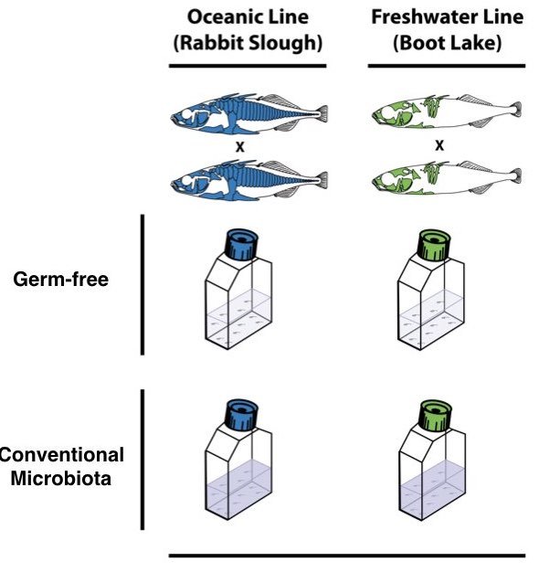{#fig-tidy-intro fig-align="center"}## What is Tidy Data?Data comes in many shapes, and not all shapes are equally convenient for analysis. The concept of "tidy data" provides a standard way to organize data that works well with R and makes many analyses straightforward. In tidy data, each variable forms a column, each observation forms a row, and each type of observational unit forms a table.{#fig-tidy-structure fig-align="center"}This structure might seem obvious, but real-world data rarely arrives in tidy form. Spreadsheets often encode information in column names, spread a single variable across multiple columns, or combine multiple variables in a single column. Data wrangling is the process of transforming messy data into tidy data.The three interrelated rules that make a dataset tidy are:1. Each variable forms a column2. Each observation forms a row3. Each type of observational unit forms a tableThese rules are interrelated because it is impossible to satisfy only two of the three. This interrelationship leads to an even simpler set of practical instructions:1. Put each dataset in a tibble (or data frame)2. Put each variable in a column## Types of DataUnderstanding the types of data you are working with guides how you analyze them and how they should be represented in R.### Categorical Data**Categorical data** classify observations into groups. There are two main types:**Nominal categorical data** have no inherent order. Examples include:- Species names (e.g., *Homo sapiens*, *Mus musculus*)- Treatment groups (control, treatment A, treatment B)- Colors (red, blue, green)- Gene names (BRCA1, TP53, EGFR)**Ordinal categorical data** have a meaningful order, but the distances between categories may not be equal. Examples include:- Ratings (low, medium, high)- Educational levels (high school, bachelor's, master's, doctorate)- Disease severity (mild, moderate, severe)- T-shirt sizes (small, medium, large, extra large)In R, categorical data are typically represented as **factors**, which store both the values and the set of possible levels. Factors are essential for statistical modeling and ensure that categories are handled consistently.### Quantitative Data**Quantitative data** are numerical measurements. Understanding the scale of measurement is important for choosing appropriate statistical tests.**Discrete quantitative data** can only take specific values, usually whole numbers:- Counts (number of offspring, number of cells)- Integers (age in years)- Scores on a fixed scale**Continuous quantitative data** can theoretically take any value within a range:- Mass, length, volume- Temperature- Concentration- Gene expression levelsQuantitative data can also be classified by their scale properties:**Interval data** have meaningful differences between values but no true zero point:- Temperature in Celsius or Fahrenheit (0° does not mean "no temperature")- Calendar dates (year 0 is arbitrary)- pH scale**Ratio data** have a true zero and meaningful ratios:- Mass, length, volume (zero means "none")- Counts (zero means "zero items")- Concentration (zero means "nothing present")- Time durationThe distinction matters because ratio data support statements like "twice as much" while interval data do not. Water at 20°C is not "twice as hot" as water at 10°C, but 20 grams is twice as heavy as 10 grams.### Data Types in RDifferent types of data are represented by different data types in R. Understanding these types helps you work with data more effectively.| Data Type | Description | Examples | R Type ||:----------|:------------|:---------|:-------|| **Character** | Text strings | "control", "treatment", gene names |`character`|| **Factor** | Categorical with levels, unordered | Species, treatment groups, colors |`factor`|| **Ordered Factor** | Categorical with meaningful order | "low" < "medium" < "high" |`ordered`|| **Integer** | Whole numbers | Count data, discrete measurements |`integer`|| **Numeric** | Real numbers (decimal) | Measurements, ratios, continuous data |`numeric` or `double`|| **Logical** | True/false values | Test results, conditions |`logical`|| **Date** | Calendar dates | "2024-01-15", sample collection dates |`Date`|| **Date-Time** | Timestamps with time | "2024-01-15 14:30:00" |`POSIXct`|You can check the type of any variable using the `class()` or `typeof()` functions:```{r}# Examples of different data typesx <-"hello"# charactery <-factor(c("A", "B", "A")) # factorz <-42# numericw <-42L # integer (the L suffix)v <-TRUE# logicald <-as.Date("2024-01-15") # Date# Check typesclass(x)class(y)class(z)typeof(z)class(w)typeof(w)class(v)class(d)```Understanding these types is crucial because:- Statistical functions expect specific data types- Categorical variables should be factors for modeling- Plotting functions treat factors differently from character strings- Mathematical operations only work on numeric types## Data File Best PracticesWhen working with data files, following consistent practices will save you time and prevent errors. These guidelines apply whether you are using Unix tools, R, or any other analysis software.### Do- **Store data in plain text formats** such as tab-separated (.tsv) or comma-separated (.csv) files. These nonproprietary formats can be read by any software and will remain accessible for years to come.- **Keep an unedited copy of original data files.** Even when your analysis requires modifications, preserve the raw data separately.- **Use descriptive, consistent names** for files and variables. A name like `experiment1_control_measurements.tsv` is far more useful than `data2.txt`.- **Maintain metadata** that documents what each variable means, how data were collected, and any processing steps applied.- **Add new observations as rows** and new variables as columns to maintain a consistent rectangular structure.- **Include a header row** with variable names that are concise but descriptive.- **Use consistent date formats**, preferably ISO 8601 format (YYYY-MM-DD).- **Represent missing values consistently**, typically as empty cells or `NA`.### Don't- **Don't mix data types within a column.** If a column contains numbers, every entry should be a number (or explicitly missing).- **Don't use special characters in file or directory names.** Stick to letters, numbers, underscores, and hyphens. Avoid spaces, which can cause problems with command-line tools.- **Don't use delimiter characters in data values.** If your file is comma-delimited, don't use commas within data entries. For example, use `2024-03-08` rather than `March 8, 2024` for dates.- **Don't copy data from formatted documents** like Microsoft Word directly into data files. Hidden formatting characters can corrupt your data.- **Don't edit data files in spreadsheet programs** that might silently convert values (for example, Excel's tendency to convert gene names like SEPT1 to dates).- **Don't use color or formatting to encode information.** All information should be in the cell values themselves, not in formatting that will be lost.- **Don't leave empty rows or columns** as visual separators. These can cause problems when reading data into analysis software.::: {.callout-warning}## Preserving Raw DataPerhaps the most important principle is to never modify your original raw data files. Keep them in a separate directory with restricted write permissions if possible. All data cleaning and transformation should be done programmatically (in scripts that can be re-run), with outputs saved to new files.:::## The TidyverseThe tidyverse is a collection of R packages designed for data science. These packages share a common philosophy and are designed to work together seamlessly. The core tidyverse packages include:- **ggplot2**: Data visualization using the grammar of graphics- **dplyr**: Data manipulation and transformation- **tidyr**: Reshaping and tidying data- **readr**: Reading rectangular data (CSV, TSV, etc.)- **purrr**: Functional programming tools- **tibble**: Enhanced data frames- **stringr**: String manipulation- **forcats**: Working with factors (categorical data)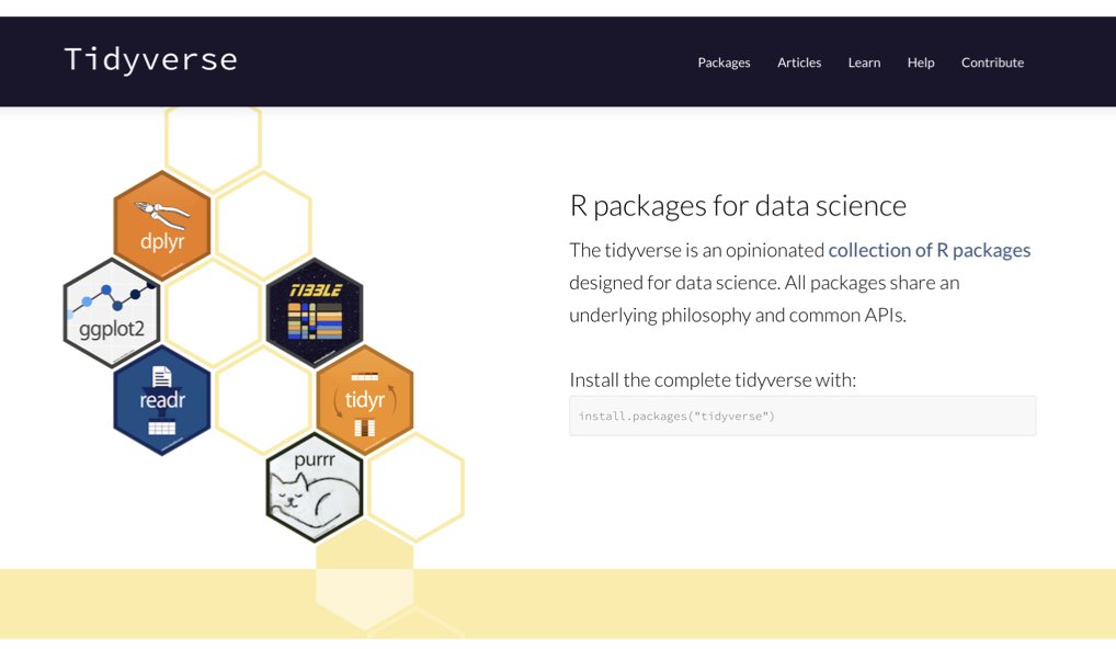{#fig-tidyverse-packages fig-align="center"}Loading the tidyverse loads all core packages at once:```{r}#| message: truelibrary(tidyverse)```The message shows which packages are attached and notes any functions that conflict with base R or other packages. For example, `dplyr::filter()` masks `stats::filter()`, meaning if you type `filter()`, you will get the dplyr version. To use the stats version, you would need to specify `stats::filter()` explicitly.## TibblesTibbles are the tidyverse's enhanced data frames. They are designed to be more user-friendly and consistent than traditional data frames, while maintaining backward compatibility for most operations.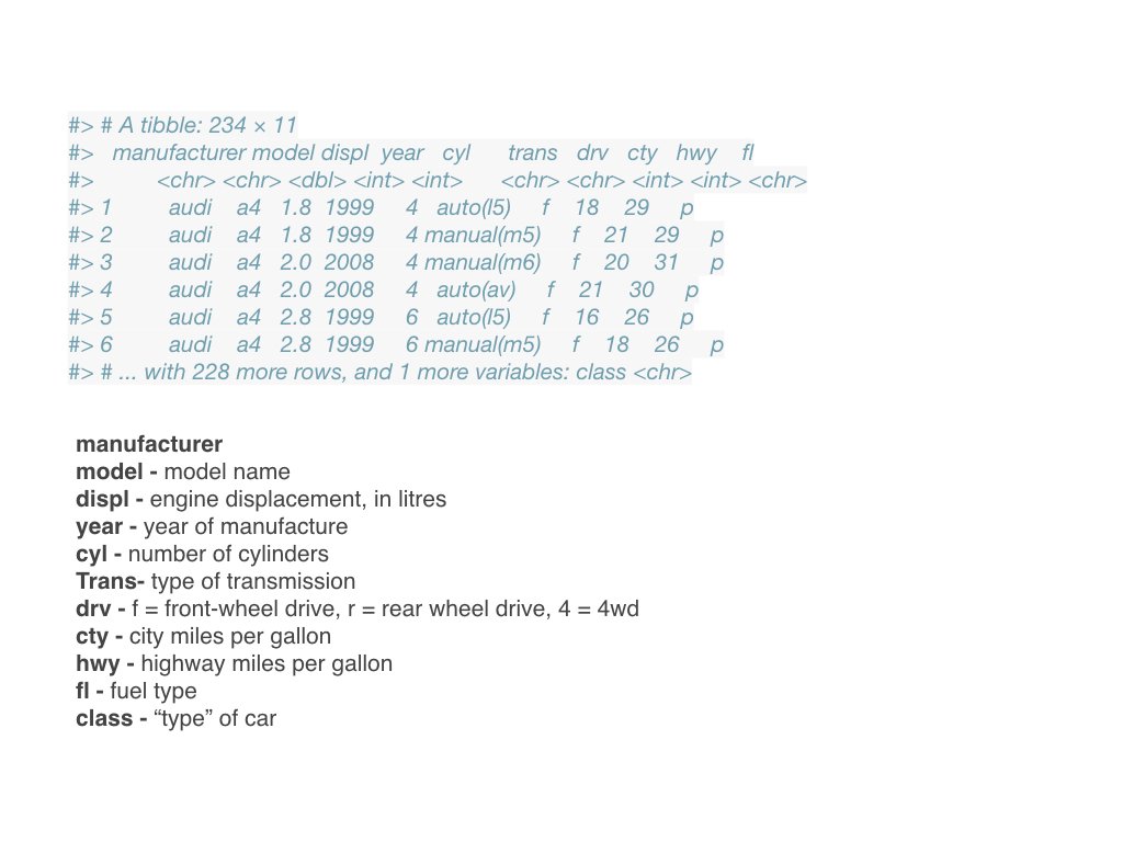{#fig-tibbles fig-align="center"}### Creating TibblesYou can create tibbles using the `tibble()` function:```{r}# Create a tibblemy_tibble <-tibble(name =c("Alice", "Bob", "Carol", "David"),age =c(25, 32, 28, 45),height_cm =c(165, 178, 172, 180),treatment =factor(c("control", "drug_A", "drug_A", "control")))my_tibble```You can also convert existing data frames to tibbles:```{r}# Convert a data frame to a tibbleiris_tibble <-as_tibble(iris)iris_tibble```### Advantages of Tibbles**Better printing**: Tibbles print more informatively than data frames. They show:- Only the first 10 rows by default- Only columns that fit on screen- The dimensions (rows × columns)- The data type of each column (shown below the column name)The column type abbreviations include:- `<chr>`: character strings- `<dbl>`: double (numeric with decimals)- `<int>`: integer- `<lgl>`: logical (TRUE/FALSE)- `<fct>`: factor- `<date>`: dates**Stricter subsetting**: Tibbles never do partial matching of names and always generate a warning if you try to access a column that doesn't exist.**No row names**: Tibbles don't use row names (they are never useful). If you have meaningful row names, convert them to a proper column.**Consistent subsetting**: `[` always returns a tibble, and `$` doesn't do partial matching.### Working with TibblesMost functions that work with data frames also work with tibbles:```{r}# Dimensionsdim(my_tibble)nrow(my_tibble)ncol(my_tibble)# Column namesnames(my_tibble)colnames(my_tibble)# Summary statisticssummary(my_tibble)```You can extract columns as vectors using `$` or `[[`:```{r}# Extract the 'name' column as a vectormy_tibble$name# Alternative syntaxmy_tibble[["name"]]```The `glimpse()` function provides a transposed summary, useful for datasets with many columns:```{r}glimpse(iris_tibble)```## Reshaping Data with tidyrSometimes data is not in the right shape for your analysis. The `tidyr` package provides functions to reshape data while maintaining tidy principles.### Wide vs. Long FormatData can be organized in wide or long format:**Wide format** has one row per subject/unit, with multiple columns for different measurements or time points:```{r}# Example: wide formatwide_data <-tibble(sample =c("A", "B", "C"),time_0 =c(10, 15, 12),time_1 =c(14, 18, 15),time_2 =c(18, 22, 19))wide_data```**Long format** has one row per observation, with variables in separate columns:```{r}# Example: long formatlong_data <-tibble(sample =c("A", "A", "A", "B", "B", "B", "C", "C", "C"),timepoint =c(0, 1, 2, 0, 1, 2, 0, 1, 2),measurement =c(10, 14, 18, 15, 18, 22, 12, 15, 19))long_data```Tidy data is typically in long format, as this structure makes it easy to:- Plot data with ggplot2 (mapping variables to aesthetics)- Group and summarize by categorical variables- Model relationships between variables### pivot_longer(): Wide to Long`pivot_longer()` takes wide data and makes it long by gathering columns into rows:```{r}# Convert wide to long formatwide_data |>pivot_longer(cols =starts_with("time_"), # which columns to pivotnames_to ="timepoint", # name for the new category columnvalues_to ="measurement"# name for the new values column )```You can also clean up the column names during the pivot:```{r}# Remove the "time_" prefix and convert to numericwide_data |>pivot_longer(cols =starts_with("time_"),names_to ="timepoint",names_prefix ="time_", # remove this prefixnames_transform = as.integer, # convert to integervalues_to ="measurement" )```### pivot_wider(): Long to Wide`pivot_wider()` does the reverse, spreading rows into columns:```{r}# Convert long to wide formatlong_data |>pivot_wider(names_from = timepoint, # which column contains new column namesvalues_from = measurement, # which column contains the valuesnames_prefix ="time_"# add prefix to new column names )```### separate(): Split One Column into Multiple`separate()` splits a single column into multiple columns:```{r}# Data with combined valuescombined_data <-tibble(sample_info =c("control_rep1", "control_rep2", "treatment_rep1", "treatment_rep2"),value =c(10, 12, 25, 23))# Separate into treatment and replicatecombined_data |>separate(col = sample_info,into =c("treatment", "replicate"),sep ="_" )```You can also separate based on character position:```{r}# Separate by positiondate_data <-tibble(date =c("20240115", "20240116"))date_data |>separate(col = date,into =c("year", "month", "day"),sep =c(4, 6) # split after positions 4 and 6 )```### unite(): Combine Multiple Columns`unite()` combines multiple columns into one:```{r}# Data with separate date componentsdate_parts <-tibble(year =c(2024, 2024, 2024),month =c(1, 2, 3),day =c(15, 20, 8))# Combine into a single date columndate_parts |>unite(col ="date", year, month, day,sep ="-" )```You can remove the original columns or keep them:```{r}# Keep original columnsdate_parts |>unite(col ="date", year, month, day,sep ="-",remove =FALSE# keep the original columns )```### Common Reshaping Patterns**Multiple measurements per subject over time** (wide to long):```{r}# Example: patient measurements at multiple time pointspatient_data <-tibble(patient_id =c("P001", "P002", "P003"),baseline =c(120, 135, 128),week_4 =c(115, 130, 125),week_8 =c(110, 125, 122))# Convert to long format for analysispatient_data |>pivot_longer(cols =-patient_id, # all columns except patient_idnames_to ="timepoint",values_to ="blood_pressure" )```**Multiple measurements of different types** (wide to long):```{r}# Example: different measurements per samplemeasurements <-tibble(sample =c("S1", "S2", "S3"),mass_g =c(2.5, 3.1, 2.8),length_mm =c(45, 52, 48),width_mm =c(12, 15, 13))# Convert to long formatmeasurements |>pivot_longer(cols =-sample,names_to =c("measurement", "unit"),names_sep ="_",values_to ="value" )```## Practice Exercises::: {.callout-note}### Exercise 7.1: Understanding Data TypesConsider the following variables from a biological experiment. For each, identify:- Whether it is categorical or quantitative- If categorical: nominal or ordinal- If quantitative: discrete or continuous, interval or ratio- What R data type would be most appropriate1. Species name (*Drosophila melanogaster*, *Caenorhabditis elegans*)2. Number of offspring produced3. Temperature in Celsius4. Treatment group (control, low dose, high dose)5. Gene expression level (measured in RPKM)6. Survival status (alive/dead)7. Tumor stage (I, II, III, IV)8. Body mass in grams9. Sample collection date10. pH level:::::: {.callout-note}### Exercise 7.2: Creating TibblesCreate a tibble with data from a hypothetical experiment:```{r}#| eval: false# Create a tibble with:# - 6 samples (S1 through S6)# - 2 treatment groups (control and experimental), 3 samples each# - A numeric measurement for each sample# - A logical variable indicating if the measurement exceeded a threshold```After creating the tibble:1. Print it and examine the column types2. Use `glimpse()` to get an overview3. Extract the measurement column as a vector4. Calculate the mean measurement for each treatment group:::::: {.callout-note}### Exercise 7.3: Reshaping DataCreate a wide-format dataset with measurements at three time points:```{r}wide_experiment <-tibble(gene =c("BRCA1", "TP53", "EGFR"),hour_0 =c(5.2, 8.1, 3.4),hour_2 =c(6.1, 8.5, 4.2),hour_4 =c(7.3, 9.2, 5.1))```1. Convert this to long format using `pivot_longer()`2. Create a new column indicating the fold-change from hour 03. Convert back to wide format, with columns for each time point's fold-change:::::: {.callout-note}### Exercise 7.4: Combining and Separating ColumnsYou have data where sample IDs encode multiple pieces of information:```{r}messy_samples <-tibble(sample_id =c("Exp1_ControlA_Rep1", "Exp1_ControlA_Rep2","Exp1_TreatmentB_Rep1", "Exp1_TreatmentB_Rep2"),measurement =c(45, 48, 62, 58))```1. Use `separate()` to split `sample_id` into: experiment, treatment, and replicate2. After analysis, use `unite()` to create a new ID combining treatment and replicate:::::: {.callout-note}### Exercise 7.5: Data File OrganizationReview a data file you have used (or create a sample one). Evaluate it against the best practices:1. Is it in plain text format?2. Does each column contain only one data type?3. Are variable names descriptive and consistent?4. Are missing values represented consistently?5. Are there any special characters that could cause problems?6. Is the data in tidy format (each variable a column, each observation a row)?If any issues exist, create a cleaned version following best practices.:::::: {.callout-note}### Exercise 7.6: Working with Real DataLoad the built-in `airquality` dataset:```{r}#| eval: falsedata(airquality)air <-as_tibble(airquality)```1. Examine the structure using `glimpse()`2. What data types are the columns?3. Convert Month to a factor with meaningful labels (e.g., "May", "June")4. The data is already in tidy format. Explain why.5. Create a wider version where each month becomes a column showing mean Ozone levels:::::: {.callout-note}### Exercise 7.7: Identifying Non-Tidy DataConsider this dataset structure:```{r}non_tidy <-tibble(gene =c("BRCA1", "TP53"),control_1 =c(5.2, 8.1),control_2 =c(5.1, 8.3),treatment_1 =c(7.3, 9.2),treatment_2 =c(7.5, 9.1))```1. Why is this not tidy data?2. What are the actual variables in this dataset?3. Reshape it into tidy format4. What are the advantages of the tidy version for analysis and visualization?:::


