Code
x <- c(2, 5, 1, 8, 3)
x
[1] 2 5 1 8 3Matrix algebra (linear algebra) is the mathematical foundation for many statistical and machine learning methods. Understanding matrices is essential for:
This appendix introduces the key concepts and R operations you need to work with matrices effectively.
A scalar is a single number. In matrix notation, scalars are typically denoted with lowercase letters:
\[a = 5, \quad b = 3.14\]
A vector is an ordered collection of numbers. In R, we create vectors with c():
x <- c(2, 5, 1, 8, 3)
x[1] 2 5 1 8 3Mathematically, we write a column vector as:
\[ \mathbf{x} = \begin{pmatrix} x_1 \\ x_2 \\ \vdots \\ x_n \end{pmatrix} \]
Vectors are typically denoted with bold lowercase letters. The transpose operation \(^\top\) converts a column vector to a row vector:
\[\mathbf{x}^\top = (x_1, x_2, \ldots, x_n)\]
A matrix is a rectangular array of numbers arranged in rows and columns. We can create matrices in R by binding vectors:
x_1 <- 1:5
x_2 <- 6:10
X <- cbind(x_1, x_2)
X
x_1 x_2
[1,] 1 6
[2,] 2 7
[3,] 3 8
[4,] 4 9
[5,] 5 10Mathematically, an \(n \times p\) matrix (n rows, p columns) is written as:
\[ \mathbf{X} = \begin{pmatrix} x_{1,1} & x_{1,2} & \cdots & x_{1,p} \\ x_{2,1} & x_{2,2} & \cdots & x_{2,p} \\ \vdots & \vdots & \ddots & \vdots \\ x_{n,1} & x_{n,2} & \cdots & x_{n,p} \end{pmatrix} \]
Matrices are denoted with bold uppercase letters. The element in row \(i\) and column \(j\) is written as \(x_{i,j}\).
The dimension of a matrix is its number of rows × number of columns:
# Load MNIST data for examples
if (!exists("mnist")) mnist <- read_mnist()
x <- mnist$train$images[1:1000, ]
y <- mnist$train$labels[1:1000]

dim(x)
[1] 1000 784This matrix has 1,000 rows (observations) and 784 columns (features—one per pixel).
nrow(x) # Number of rows[1] 1000ncol(x) # Number of columns[1] 784R vectors don’t have dimensions:
v <- 1:5
dim(v)NULLTo treat a vector as a matrix, use as.matrix():
dim(as.matrix(v))[1] 5 1matrix() FunctionCreate a matrix from a vector by specifying dimensions:
my_vector <- 1:12
mat <- matrix(my_vector, nrow = 3, ncol = 4)
mat
[,1] [,2] [,3] [,4]
[1,] 1 4 7 10
[2,] 2 5 8 11
[3,] 3 6 9 12By default, matrices are filled by column. Use byrow = TRUE to fill by row:
mat_byrow <- matrix(my_vector, nrow = 3, ncol = 4, byrow = TRUE)
mat_byrow
[,1] [,2] [,3] [,4]
[1,] 1 2 3 4
[2,] 5 6 7 8
[3,] 9 10 11 12A powerful application is reshaping a vector into a 2D image. Each row of the MNIST data is a 784-element vector representing a 28×28 pixel image:
# Convert the 3rd digit to a grid
grid <- matrix(x[3, ], 28, 28)

# Display (flip to show correctly)
image(1:28, 1:28, grid[, 28:1], col = gray.colors(256, start = 1, end = 0),
      xlab = "", ylab = "", main = paste("Digit:", y[3]))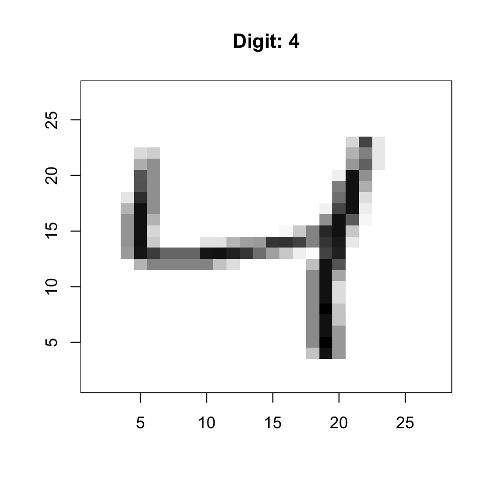
The transpose swaps rows and columns:
mat <- matrix(1:6, nrow = 2, ncol = 3)
mat
[,1] [,2] [,3]
[1,] 1 3 5
[2,] 2 4 6t(mat) [,1] [,2]
[1,] 1 2
[2,] 3 4
[3,] 5 6Use [row, column] notation:
mat <- matrix(1:12, nrow = 3, ncol = 4)

# Single element
mat[2, 3]
[1] 8# Entire row
mat[2, ][1] 2 5 8 11# Entire column
mat[, 3][1] 7 8 9# Multiple rows/columns
mat[1:2, 3:4] [,1] [,2]
[1,] 7 10
[2,] 8 11Extracting a single row or column returns a vector by default:
class(mat[, 1])[1] "integer"Use drop = FALSE to keep it as a matrix:
class(mat[, 1, drop = FALSE])[1] "matrix" "array" Select elements based on conditions:
mat <- matrix(1:12, nrow = 3, ncol = 4)
mat[mat > 6] <- 0  # Set values > 6 to zero
mat
[,1] [,2] [,3] [,4]
[1,] 1 4 0 0
[2,] 2 5 0 0
[3,] 3 6 0 0This is useful for operations like binarizing data:
# Binarize MNIST data (convert to 0/1)
bin_x <- (x > 127) * 1Compute summaries across rows or columns:
# Row sums and means
row_sums <- rowSums(x)
row_means <- rowMeans(x)

# Column sums and means
col_sums <- colSums(x)
col_means <- colMeans(x)
For standard deviations, use the matrixStats package:
library(matrixStats)
row_sds <- rowSds(x)
col_sds <- colSds(x)apply() FunctionApply any function across rows (margin = 1) or columns (margin = 2):
# Row medians
row_medians <- apply(x, 1, median)

# Column ranges
col_ranges <- apply(x, 2, function(col) max(col) - min(col))Remove low-variance columns (uninformative pixels):
# Keep only columns with SD > 60
sds <- colSds(x)
x_filtered <- x[, sds > 60]
dim(x_filtered)
[1] 1000 314This removes over half the predictors while keeping informative features.
Standard arithmetic operates element-by-element:
A <- matrix(1:4, 2, 2)
B <- matrix(5:8, 2, 2)

A + B   # Addition
[,1] [,2]
[1,] 6 10
[2,] 8 12A * B # Element-wise multiplication [,1] [,2]
[1,] 5 21
[2,] 12 32A / B # Element-wise division [,1] [,2]
[1,] 0.2000000 0.4285714
[2,] 0.3333333 0.5000000When operating with vectors, R recycles along columns:
mat <- matrix(1:6, nrow = 2, ncol = 3)
vec <- c(10, 20)
mat + vec  # Adds 10 to row 1, 20 to row 2
[,1] [,2] [,3]
[1,] 11 13 15
[2,] 22 24 26sweep() FunctionFor more control over row/column operations:
# Subtract column means (center the data)
x_centered <- sweep(x, 2, colMeans(x))

# Divide by column SDs (standardize)
x_standardized <- sweep(x_centered, 2, colSds(x), FUN = "/")
For row operations, use margin = 1:
# Subtract row means
x_row_centered <- sweep(x, 1, rowMeans(x))Matrix multiplication is not element-wise. For matrices \(\mathbf{A}\) (\(n \times k\)) and \(\mathbf{B}\) (\(k \times p\)), the product \(\mathbf{C} = \mathbf{AB}\) is an \(n \times p\) matrix where:
\[c_{i,j} = \sum_{l=1}^{k} a_{i,l} \cdot b_{l,j}\]
The number of columns in \(\mathbf{A}\) must equal the number of rows in \(\mathbf{B}\).
In R, use %*% for matrix multiplication:
A <- matrix(1:6, nrow = 2, ncol = 3)
B <- matrix(1:6, nrow = 3, ncol = 2)

A %*% B
[,1] [,2]
[1,] 22 49
[2,] 28 64The cross product \(\mathbf{X}^\top\mathbf{X}\) is fundamental in statistics:
# Using matrix multiplication
XtX <- t(x) %*% x

# More efficient built-in function
XtX <- crossprod(x)
The cross product creates a \(p \times p\) matrix where element \((i,j)\) is the dot product of columns \(i\) and \(j\).
Multiplying a matrix by a vector transforms the vector:
A <- matrix(c(2, 0, 0, 3), nrow = 2)  # Scaling matrix
v <- c(1, 1)
A %*% v
[,1]
[1,] 2
[2,] 3This concept is central to understanding eigenanalysis and PCA.
For centered data \(\mathbf{X}\) (column means = 0), the covariance matrix is:
\[\mathbf{\Sigma} = \frac{1}{n-1} \mathbf{X}^\top \mathbf{X}\]
# Center the data
x_centered <- scale(x, center = TRUE, scale = FALSE)

# Compute covariance matrix
cov_matrix <- cov(x_centered)
dim(cov_matrix)
[1] 784 784The covariance matrix is: - Symmetric: \(\Sigma_{ij} = \Sigma_{ji}\) - Positive semi-definite: All eigenvalues ≥ 0 - Diagonal elements: Variances of each variable - Off-diagonal elements: Covariances between variables
Eigenanalysis is the mathematical foundation of Principal Component Analysis (PCA). Understanding eigenvalues and eigenvectors helps you interpret PCA results correctly.
For a square matrix \(\mathbf{A}\), an eigenvector \(\mathbf{v}\) and its corresponding eigenvalue \(\lambda\) satisfy:
\[\mathbf{A}\mathbf{v} = \lambda\mathbf{v}\]
This equation says that when we multiply \(\mathbf{A}\) by \(\mathbf{v}\), the result is just \(\mathbf{v}\) scaled by \(\lambda\). The eigenvector’s direction doesn’t change—only its magnitude.
Most vectors change direction when multiplied by a matrix. Eigenvectors are special—they only get stretched or compressed:
# Define a transformation matrix
A <- matrix(c(2, 1, 1, 2), nrow = 2)

# Compute eigenvectors
eig <- eigen(A)

# Regular vector (changes direction)
v_regular <- c(1, 0)
v_transformed <- A %*% v_regular

# Eigenvector (only scales)
v_eigen <- eig$vectors[, 1]
v_eigen_transformed <- A %*% v_eigen

# Plot
plot(NULL, xlim = c(-3, 3), ylim = c(-3, 3), asp = 1,
     xlab = "x", ylab = "y", main = "Eigenvector vs Regular Vector")
abline(h = 0, v = 0, col = "gray80")

# Regular vector and its transform
arrows(0, 0, v_regular[1], v_regular[2], col = "blue", lwd = 2)
arrows(0, 0, v_transformed[1], v_transformed[2], col = "blue", lwd = 2, lty = 2)

# Eigenvector and its transform
arrows(0, 0, v_eigen[1], v_eigen[2], col = "red", lwd = 2)
arrows(0, 0, v_eigen_transformed[1], v_eigen_transformed[2], col = "red", lwd = 2, lty = 2)

legend("topleft", c("Regular (original)", "Regular (transformed)",
                    "Eigenvector (original)", "Eigenvector (transformed)"),
       col = c("blue", "blue", "red", "red"), lty = c(1, 2, 1, 2), lwd = 2)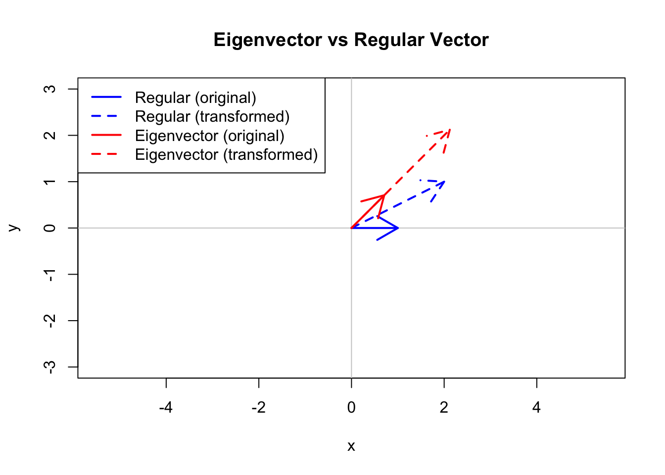
# Symmetric matrix example
A <- matrix(c(4, 2, 2, 3), nrow = 2)
eig <- eigen(A)

# Eigenvalues
eig$values
[1] 5.561553 1.438447# Eigenvectors (as columns)
eig$vectors [,1] [,2]
[1,] -0.7882054 0.6154122
[2,] -0.6154122 -0.7882054Verify the eigenvalue equation \(\mathbf{A}\mathbf{v} = \lambda\mathbf{v}\):
v1 <- eig$vectors[, 1]
lambda1 <- eig$values[1]

# These should be equal
A %*% v1
[,1]
[1,] -4.383646
[2,] -3.422648lambda1 * v1[1] -4.383646 -3.422648For symmetric matrices (like covariance matrices):
# Verify orthogonality: dot product = 0
sum(eig$vectors[, 1] * eig$vectors[, 2])
[1] 0PCA performs eigenanalysis on the covariance (or correlation) matrix. Here’s the connection:
# Simple example with iris data
iris_centered <- scale(iris[, 1:4], center = TRUE, scale = FALSE)
cov_iris <- cov(iris_centered)

# Eigenanalysis
eig_iris <- eigen(cov_iris)

# Compare to PCA
pca_iris <- prcomp(iris[, 1:4], center = TRUE, scale. = FALSE)

# Eigenvalues = squared singular values = variances
eig_iris$values
[1] 4.22824171 0.24267075 0.07820950 0.02383509pca_iris$sdev^2[1] 4.22824171 0.24267075 0.07820950 0.02383509The loadings from PCA match the eigenvectors (possibly with sign flips, which are arbitrary):
# Eigenvectors
round(eig_iris$vectors, 3)
[,1] [,2] [,3] [,4]
[1,] 0.361 -0.657 -0.582 0.315
[2,] -0.085 -0.730 0.598 -0.320
[3,] 0.857 0.173 0.076 -0.480
[4,] 0.358 0.075 0.546 0.754# PCA loadings
round(pca_iris$rotation, 3) PC1 PC2 PC3 PC4
Sepal.Length 0.361 -0.657 0.582 0.315
Sepal.Width -0.085 -0.730 -0.598 -0.320
Petal.Length 0.857 0.173 -0.076 -0.480
Petal.Width 0.358 0.075 -0.546 0.754Eigenvalues tell you how much variance each principal component captures.
# Compute proportion of variance
var_explained <- eig_iris$values / sum(eig_iris$values)
cumulative_var <- cumsum(var_explained)

par(mfrow = c(1, 2))
barplot(var_explained * 100, names.arg = paste0("PC", 1:4),
        ylab = "Variance Explained (%)", main = "Individual Variance")

barplot(cumulative_var * 100, names.arg = paste0("PC", 1:4),
        ylab = "Cumulative Variance (%)", main = "Cumulative Variance")
abline(h = 90, col = "red", lty = 2)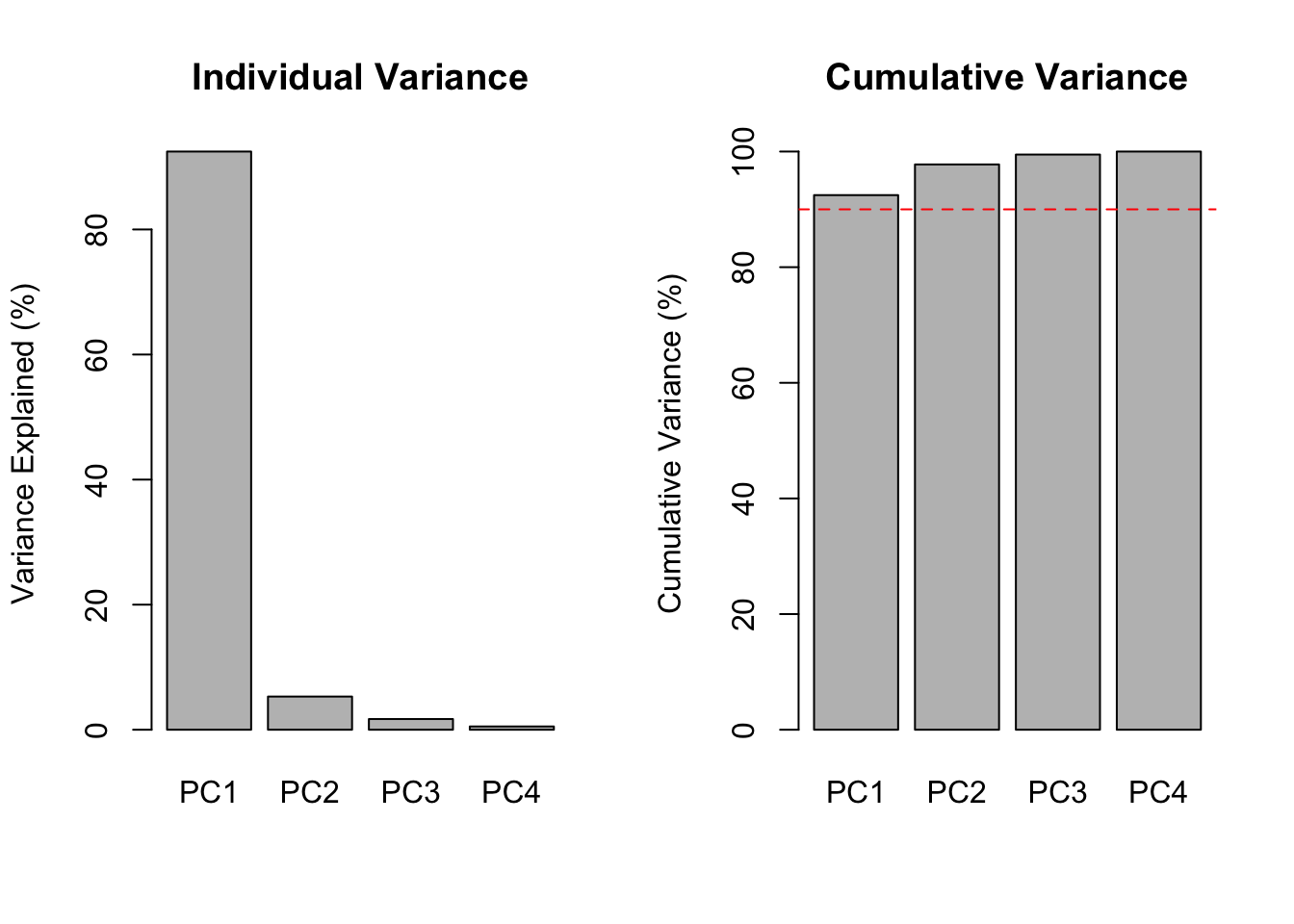
Key interpretations:
Eigenvectors tell you how original variables combine to form each PC.
loadings_df <- data.frame(
  Variable = rep(colnames(iris)[1:4], 4),
  PC = rep(paste0("PC", 1:4), each = 4),
  Loading = as.vector(pca_iris$rotation)
)

ggplot(loadings_df, aes(x = Variable, y = Loading, fill = Loading > 0)) +
  geom_bar(stat = "identity") +
  facet_wrap(~PC, nrow = 1) +
  scale_fill_manual(values = c("steelblue", "coral"), guide = "none") +
  theme(axis.text.x = element_text(angle = 45, hjust = 1)) +
  labs(title = "PCA Loadings for Iris Data")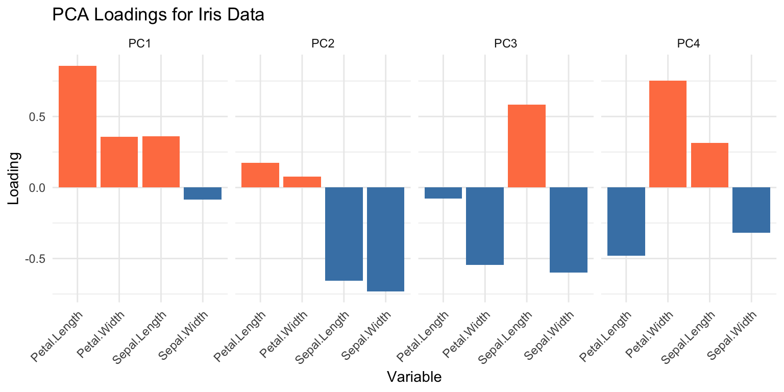
Key interpretations:
A symmetric matrix can be decomposed as:
\[\mathbf{A} = \mathbf{V} \mathbf{\Lambda} \mathbf{V}^\top\]
where: - \(\mathbf{V}\) is the matrix of eigenvectors (columns) - \(\mathbf{\Lambda}\) is a diagonal matrix of eigenvalues
# Verify spectral decomposition
V <- eig_iris$vectors
Lambda <- diag(eig_iris$values)
reconstructed <- V %*% Lambda %*% t(V)

# Should match original covariance matrix
max(abs(cov_iris - reconstructed))
[1] 8.881784e-16This decomposition is the mathematical basis for PCA’s ability to reduce dimensionality while preserving variance.
The inverse of a square matrix \(\mathbf{A}\), denoted \(\mathbf{A}^{-1}\), satisfies:
\[\mathbf{A}\mathbf{A}^{-1} = \mathbf{A}^{-1}\mathbf{A} = \mathbf{I}\]
where \(\mathbf{I}\) is the identity matrix.
A <- matrix(c(4, 2, 2, 3), nrow = 2)
A_inv <- solve(A)

# Verify
A %*% A_inv
[,1] [,2]
[1,] 1 0
[2,] 0 1Matrix inversion is used in:
# Solve linear system Ax = b
A <- matrix(c(2, 1, 1, 3), nrow = 2)
b <- c(5, 7)
x <- solve(A, b)  # More efficient than solve(A) %*% b
x
[1] 1.6 1.8# Verify
A %*% x [,1]
[1,] 5
[2,] 7The QR decomposition factors a matrix as \(\mathbf{X} = \mathbf{QR}\) where:
This is numerically more stable than matrix inversion for solving linear systems.
qr_result <- qr(A)
Q <- qr.Q(qr_result)
R <- qr.R(qr_result)

# Verify
Q %*% R
[,1] [,2]
[1,] 2 1
[2,] 1 3Key matrix algebra concepts for statistics:
| Operation | R Function | Description |
|---|---|---|
| Transpose | t(X) |
Swap rows and columns |
| Matrix multiply | X %*% Y |
Matrix multiplication |
| Cross product | crossprod(X) |
\(\mathbf{X}^\top\mathbf{X}\) |
| Element-wise ops | X * Y, X + Y |
Apply to each element |
| Row/column stats | rowMeans(), colSds() |
Summary statistics |
| Standardize | sweep(), scale() |
Center and scale |
| Eigenanalysis | eigen() |
Eigenvalues and eigenvectors |
| Inverse | solve() |
Matrix inverse |
| QR decomposition | qr() |
Orthogonal decomposition |
For PCA (see Chapter 37):
Create a 100 × 10 matrix of randomly generated normal numbers. Compute its dimensions, number of rows, and number of columns.
Add the scalar 1 to row 1, the scalar 2 to row 2, and so on, to the matrix from Exercise 1. Hint: create a vector 1:100 and add it.
Perform eigenanalysis on the iris covariance matrix. Which variable contributes most to PC1?
Verify that the eigenvectors are orthogonal by computing their pairwise dot products.
sweep().