26 Multiple Regression

26.1 Beyond One Predictor

Simple linear regression uses a single predictor. But the response variable often depends on multiple factors. A patient’s blood pressure might depend on age, weight, sodium intake, and medication. Gene expression might depend on temperature, time, and treatment condition.

Multiple regression extends linear regression to multiple predictors:

\[y_i = \beta_0 + \beta_1 x_1 + \beta_2 x_2 + \ldots + \beta_p x_p + \epsilon_i\]

26.2 Goals of Multiple Regression

Multiple regression serves two main purposes. First, it often improves prediction by incorporating multiple sources of information. Second, it allows us to investigate the effect of each predictor while controlling for the others—the effect of X1 “holding X2 constant.”

This second goal is powerful but requires caution. In observational data, controlling for variables statistically is not the same as controlling them experimentally. Confounding variables you do not measure cannot be controlled.

26.3 Understanding Confounding Through Stratification

A powerful way to understand confounding—and why multiple regression is necessary—is through stratification. When two predictors are correlated, their apparent individual effects can be misleading.

Consider a biological example: suppose we measure both body size and metabolic rate in animals, and we want to know if each independently predicts lifespan. If larger animals have both higher metabolic rates AND longer lifespans (because both correlate with species type), we might see a spurious positive relationship between metabolic rate and lifespan when the true relationship is negative within any given body size.

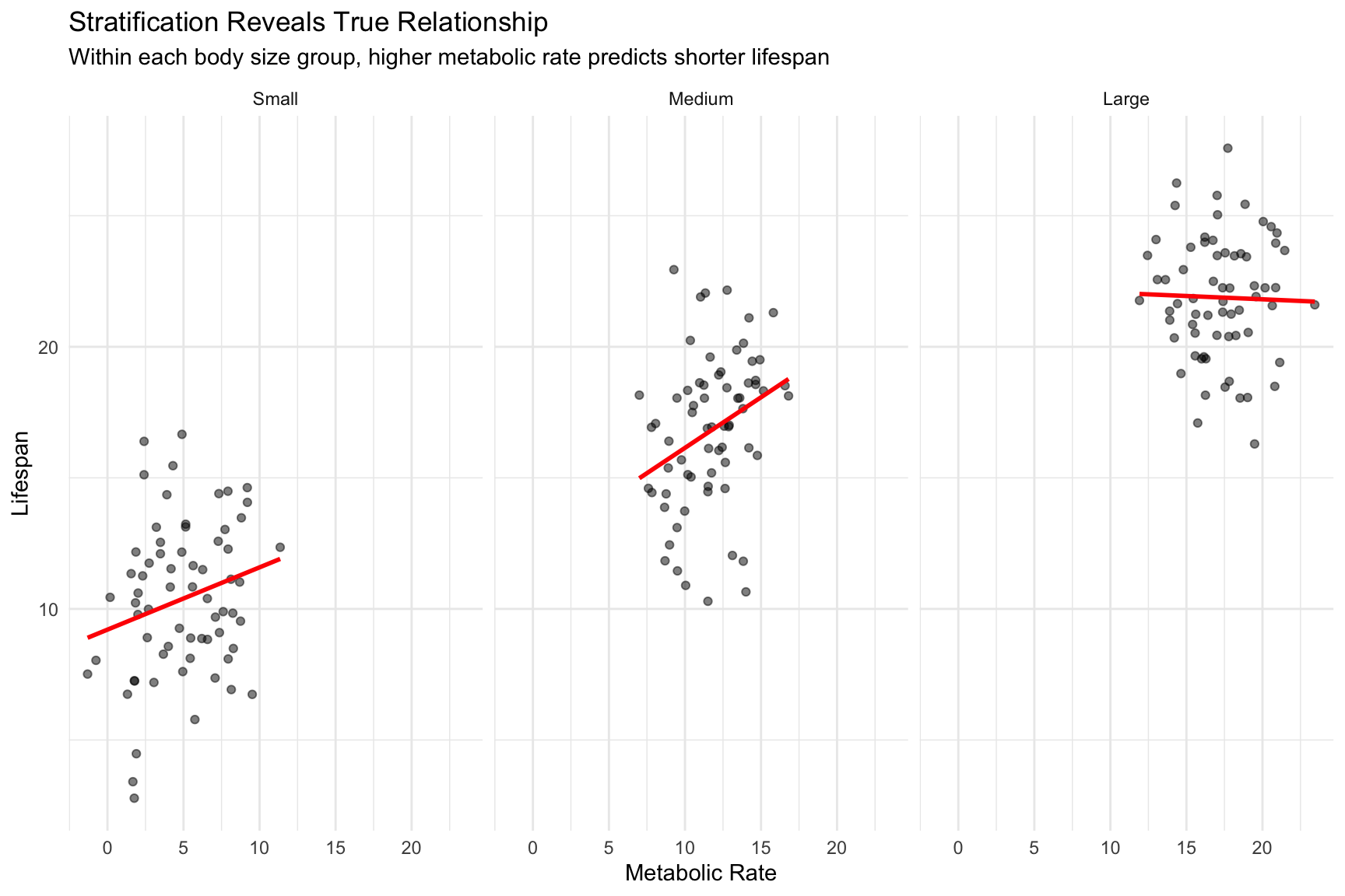
The solution is to stratify by the confounding variable. If we group animals by body size and look at the relationship between metabolic rate and lifespan within each group, we see the true (negative) relationship.

Code

# Simulated confounding example
set.seed(42)
n <- 200

# Body size (the confounder)
body_size <- runif(n, 1, 10)

# Metabolic rate increases with body size (positive correlation with confounder)
metabolic_rate <- 2 * body_size + rnorm(n, sd = 2)

# Lifespan: increases with body size, DECREASES with metabolic rate
# But without controlling for body size, it appears metabolic rate increases lifespan!
lifespan <- 5 + 3 * body_size - 0.5 * metabolic_rate + rnorm(n, sd = 2)

confound_data <- data.frame(body_size, metabolic_rate, lifespan)

# Naive regression (ignoring confounder)
naive_fit <- lm(lifespan ~ metabolic_rate, data = confound_data)

# Proper multiple regression (controlling for body size)
proper_fit <- lm(lifespan ~ metabolic_rate + body_size, data = confound_data)

cat("Naive model (ignoring body size):\n")

Naive model (ignoring body size):

Code

cat("Metabolic rate coefficient:", round(coef(naive_fit)[2], 3), "\n\n")

Metabolic rate coefficient: 0.787

Code

cat("Multiple regression (controlling for body size):\n")

Multiple regression (controlling for body size):

Code

cat("Metabolic rate coefficient:", round(coef(proper_fit)[2], 3), "\n")

Metabolic rate coefficient: -0.466

Code

cat("Body size coefficient:", round(coef(proper_fit)[3], 3), "\n")

Body size coefficient: 2.844

The naive model shows a positive relationship between metabolic rate and lifespan. But once we control for body size, we see the true negative relationship—higher metabolic rate is associated with shorter lifespan, as biological theory predicts.

We can visualize this confounding through stratification:

Code

# Stratify by body size
confound_data$size_strata <- cut(confound_data$body_size,
                                  breaks = quantile(body_size, c(0, 0.33, 0.67, 1)),
                                  labels = c("Small", "Medium", "Large"),
                                  include.lowest = TRUE)

# Plot relationship within each stratum
ggplot(confound_data, aes(x = metabolic_rate, y = lifespan)) +
  geom_point(alpha = 0.5) +
  geom_smooth(method = "lm", se = FALSE, color = "red") +
  facet_wrap(~ size_strata) +
  labs(title = "Stratification Reveals True Relationship",
       subtitle = "Within each body size group, higher metabolic rate predicts shorter lifespan",
       x = "Metabolic Rate", y = "Lifespan") +
  theme_minimal()

Figure 26.2: Stratification by body size reveals the true negative relationship between metabolic rate and lifespan

Within each stratum (holding body size approximately constant), we see the true negative relationship. The slopes within strata approximate what multiple regression gives us.

Simpson’s Paradox

This phenomenon—where a trend reverses or disappears when data are stratified by a confounding variable—is known as Simpson’s Paradox. In our example, metabolic rate appears positively associated with lifespan in the aggregate data, but is negatively associated within each body size group.

Simpson’s Paradox is not a statistical anomaly; it’s a consequence of confounding. Famous examples include:

UC Berkeley gender bias case (1973): Aggregate admission rates appeared to favor men, but within most departments, women were admitted at equal or higher rates. The paradox arose because women disproportionately applied to more competitive departments.
Kidney stone treatments: Treatment A appeared less effective overall, but was more effective for both small and large stones. The paradox occurred because Treatment A was preferentially used for more severe cases.

The resolution is always the same: aggregate data can be misleading when a confounding variable affects both the predictor and outcome. Stratification (or multiple regression) reveals the relationship within levels of the confounder.

Why This Matters

When predictors are correlated, simple regression coefficients can be misleading—even showing the wrong sign! Multiple regression “adjusts” for confounders, revealing relationships that are closer to (though not necessarily equal to) causal effects. However, you can only adjust for confounders you measure. Unmeasured confounders remain a threat to causal interpretation.

26.4 Additive vs. Multiplicative Models

An additive model assumes predictors contribute independently:

\[y = \beta_0 + \beta_1 x_1 + \beta_2 x_2 + \epsilon\]

A multiplicative model includes interactions—the effect of one predictor depends on the value of another:

\[y = \beta_0 + \beta_1 x_1 + \beta_2 x_2 + \beta_3 x_1 x_2 + \epsilon\]

Code

# Example with two predictors
set.seed(42)
n <- 100
x1 <- rnorm(n)
x2 <- rnorm(n)
y <- 2 + 3*x1 + 2*x2 + 1.5*x1*x2 + rnorm(n)

# Additive model
add_model <- lm(y ~ x1 + x2)

# Model with interaction
int_model <- lm(y ~ x1 * x2)

summary(int_model)


Call:
lm(formula = y ~ x1 * x2)

Residuals:
     Min       1Q   Median       3Q      Max 
-2.55125 -0.69885 -0.03771  0.56441  2.42157 

Coefficients:
            Estimate Std. Error t value Pr(>|t|)    
(Intercept)  2.00219    0.10108   19.81   <2e-16 ***
x1           2.84494    0.09734   29.23   <2e-16 ***
x2           2.04126    0.11512   17.73   <2e-16 ***
x1:x2        1.35163    0.09228   14.65   <2e-16 ***
---
Signif. codes:  0 '***' 0.001 '**' 0.01 '*' 0.05 '.' 0.1 ' ' 1

Residual standard error: 1.005 on 96 degrees of freedom
Multiple R-squared:  0.9289,    Adjusted R-squared:  0.9267 
F-statistic:   418 on 3 and 96 DF,  p-value: < 2.2e-16

26.5 Interpretation of Coefficients

In multiple regression, each coefficient represents the expected change in Y for a one-unit change in that predictor, holding all other predictors constant.

This “holding constant” interpretation makes the coefficients different from what you would get from separate simple regressions. The coefficient for X1 in multiple regression represents the unique contribution of X1 after accounting for X2.

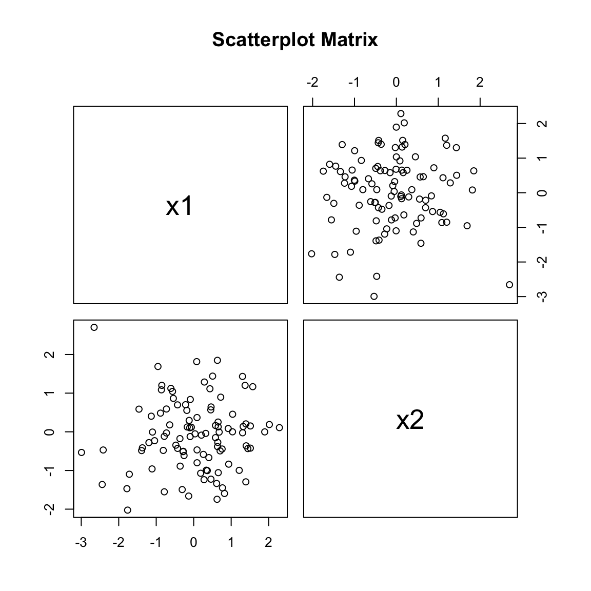
26.6 Multicollinearity

When predictors are correlated with each other, interpreting individual coefficients becomes problematic. This multicollinearity inflates standard errors and can make coefficients unstable.

Code

# Check for multicollinearity visually
library(car)
pairs(~ x1 + x2, main = "Scatterplot Matrix")

Figure 26.3: Scatterplot matrix for checking multicollinearity between predictors

The Variance Inflation Factor (VIF) quantifies multicollinearity. VIF > 10 suggests serious problems; VIF > 5 warrants attention.

Code

vif(int_model)

      x1       x2    x1:x2 
1.006276 1.061022 1.066455

26.7 Model Selection

With many potential predictors, how do we choose which to include? Adding variables always improves fit to the training data but may hurt prediction on new data through overfitting.

Several criteria balance fit and complexity:

Adjusted R² penalizes for the number of predictors.

AIC (Akaike Information Criterion) estimates prediction error, penalizing complexity. Lower is better.

BIC (Bayesian Information Criterion) similar to AIC but penalizes complexity more heavily.

Code

# Compare models
AIC(add_model, int_model)

          df      AIC
add_model  4 406.1808
int_model  5 290.7926

Code

BIC(add_model, int_model)

          df      BIC
add_model  4 416.6015
int_model  5 303.8185

26.8 Model Selection Strategies

Forward selection starts with no predictors and adds them one at a time based on statistical criteria.

Backward elimination starts with all predictors and removes them one at a time.

All subsets examines all possible combinations and selects the best.

No strategy is universally best. Automated selection can lead to overfitting and unstable models. Theory-driven model building—starting with predictors you have scientific reasons to include—is often preferable.

26.9 Polynomial Regression

Polynomial terms can capture non-linear relationships while still using the linear regression framework:

Code

# Non-linear relationship
x <- seq(0, 10, length.out = 100)
y <- 2 + 0.5*x - 0.1*x^2 + rnorm(100, sd = 0.5)

# Fit polynomial models
model1 <- lm(y ~ poly(x, 1))  # Linear
model2 <- lm(y ~ poly(x, 2))  # Quadratic
model3 <- lm(y ~ poly(x, 5))  # Degree 5

# Compare
AIC(model1, model2, model3)

       df      AIC
model1  3 250.3022
model2  4 121.8041
model3  7 126.6399

Higher-degree polynomials fit better but risk overfitting. The principle of parsimony suggests using the simplest adequate model.

Figure 26.4: Illustration of polynomial regression showing increasing model complexity

26.10 Assumptions

Multiple regression shares assumptions with simple regression: linearity (in each predictor), independence, normality of residuals, and constant variance. Additionally, predictors should not be perfectly correlated (no perfect multicollinearity).

Check assumptions with residual plots. Partial regression plots can help diagnose problems with individual predictors.

26.11 Practical Guidelines

Start with a theoretically motivated model rather than throwing in all available predictors. Check for multicollinearity before interpreting coefficients. Use cross-validation to assess prediction performance. Report standardized coefficients when comparing the relative importance of predictors on different scales.

Be humble about causation. Multiple regression describes associations; experimental manipulation is needed to establish causation.

# Multiple Regression {#sec-multiple-regression} ```{r} #| echo: false #| message: false library(tidyverse) theme_set(theme_minimal()) ``` ## Beyond One Predictor Simple linear regression uses a single predictor. But the response variable often depends on multiple factors. A patient's blood pressure might depend on age, weight, sodium intake, and medication. Gene expression might depend on temperature, time, and treatment condition. Multiple regression extends linear regression to multiple predictors: $$y_i = \beta_0 + \beta_1 x_1 + \beta_2 x_2 + \ldots + \beta_p x_p + \epsilon_i$$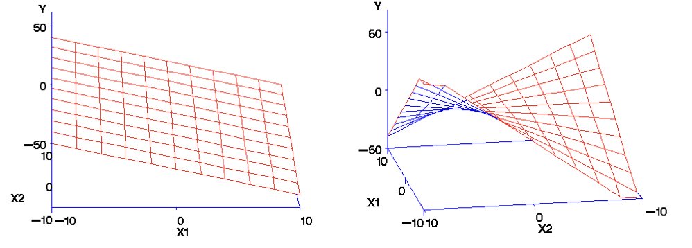 ![Multiple regression extends linear regression to multiple predictors in multidimensional space](../images/ch24/ch24_multiple_regression.jpeg){#fig-multiple-regression-concept fig-align="center"} ## Goals of Multiple Regression Multiple regression serves two main purposes. First, it often improves prediction by incorporating multiple sources of information. Second, it allows us to investigate the effect of each predictor while controlling for the others—the effect of X1 "holding X2 constant." This second goal is powerful but requires caution. In observational data, controlling for variables statistically is not the same as controlling them experimentally. Confounding variables you do not measure cannot be controlled. ## Understanding Confounding Through Stratification A powerful way to understand confounding—and why multiple regression is necessary—is through stratification. When two predictors are correlated, their apparent individual effects can be misleading. Consider a biological example: suppose we measure both body size and metabolic rate in animals, and we want to know if each independently predicts lifespan. If larger animals have both higher metabolic rates AND longer lifespans (because both correlate with species type), we might see a spurious positive relationship between metabolic rate and lifespan when the true relationship is negative within any given body size. The solution is to **stratify** by the confounding variable. If we group animals by body size and look at the relationship between metabolic rate and lifespan within each group, we see the true (negative) relationship. ```{r} #| label: fig-confounding-example #| fig-cap: "Demonstration of confounding: naive versus multiple regression coefficients" #| fig-width: 8 #| fig-height: 6 # Simulated confounding example set.seed(42) n <- 200 # Body size (the confounder) body_size <- runif(n, 1, 10) # Metabolic rate increases with body size (positive correlation with confounder) metabolic_rate <- 2 * body_size + rnorm(n, sd = 2) # Lifespan: increases with body size, DECREASES with metabolic rate # But without controlling for body size, it appears metabolic rate increases lifespan! lifespan <- 5 + 3 * body_size - 0.5 * metabolic_rate + rnorm(n, sd = 2) confound_data <- data.frame(body_size, metabolic_rate, lifespan) # Naive regression (ignoring confounder) naive_fit <- lm(lifespan ~ metabolic_rate, data = confound_data) # Proper multiple regression (controlling for body size) proper_fit <- lm(lifespan ~ metabolic_rate + body_size, data = confound_data) cat("Naive model (ignoring body size):\n") cat("Metabolic rate coefficient:", round(coef(naive_fit)[2], 3), "\n\n") cat("Multiple regression (controlling for body size):\n") cat("Metabolic rate coefficient:", round(coef(proper_fit)[2], 3), "\n") cat("Body size coefficient:", round(coef(proper_fit)[3], 3), "\n") ``` The naive model shows a *positive* relationship between metabolic rate and lifespan. But once we control for body size, we see the true *negative* relationship—higher metabolic rate is associated with shorter lifespan, as biological theory predicts. We can visualize this confounding through stratification: ```{r} #| label: fig-stratification #| fig-cap: "Stratification by body size reveals the true negative relationship between metabolic rate and lifespan" #| fig-width: 9 #| fig-height: 6 # Stratify by body size confound_data$size_strata <- cut(confound_data$body_size, breaks = quantile(body_size, c(0, 0.33, 0.67, 1)), labels = c("Small", "Medium", "Large"), include.lowest = TRUE) # Plot relationship within each stratum ggplot(confound_data, aes(x = metabolic_rate, y = lifespan)) + geom_point(alpha = 0.5) + geom_smooth(method = "lm", se = FALSE, color = "red") + facet_wrap(~ size_strata) + labs(title = "Stratification Reveals True Relationship", subtitle = "Within each body size group, higher metabolic rate predicts shorter lifespan", x = "Metabolic Rate", y = "Lifespan") + theme_minimal() ``` Within each stratum (holding body size approximately constant), we see the true negative relationship. The slopes within strata approximate what multiple regression gives us. ::: {.callout-note} ## Simpson's Paradox This phenomenon—where a trend reverses or disappears when data are stratified by a confounding variable—is known as **Simpson's Paradox**. In our example, metabolic rate appears *positively* associated with lifespan in the aggregate data, but is *negatively* associated within each body size group. Simpson's Paradox is not a statistical anomaly; it's a consequence of confounding. Famous examples include: - **UC Berkeley gender bias case (1973)**: Aggregate admission rates appeared to favor men, but within most departments, women were admitted at equal or higher rates. The paradox arose because women disproportionately applied to more competitive departments. - **Kidney stone treatments**: Treatment A appeared less effective overall, but was more effective for both small and large stones. The paradox occurred because Treatment A was preferentially used for more severe cases. The resolution is always the same: aggregate data can be misleading when a confounding variable affects both the predictor and outcome. Stratification (or multiple regression) reveals the relationship within levels of the confounder. ::: ::: {.callout-important} ## Why This Matters When predictors are correlated, simple regression coefficients can be misleading—even showing the wrong sign! Multiple regression "adjusts" for confounders, revealing relationships that are closer to (though not necessarily equal to) causal effects. However, you can only adjust for confounders you measure. Unmeasured confounders remain a threat to causal interpretation. ::: ## Additive vs. Multiplicative Models An **additive model** assumes predictors contribute independently: $$y = \beta_0 + \beta_1 x_1 + \beta_2 x_2 + \epsilon$$ A **multiplicative model** includes interactions—the effect of one predictor depends on the value of another: $$y = \beta_0 + \beta_1 x_1 + \beta_2 x_2 + \beta_3 x_1 x_2 + \epsilon$$ ```{r} # Example with two predictors set.seed(42) n <- 100 x1 <- rnorm(n) x2 <- rnorm(n) y <- 2 + 3*x1 + 2*x2 + 1.5*x1*x2 + rnorm(n) # Additive model add_model <- lm(y ~ x1 + x2) # Model with interaction int_model <- lm(y ~ x1 * x2) summary(int_model) ``` ## Interpretation of Coefficients In multiple regression, each coefficient represents the expected change in Y for a one-unit change in that predictor, **holding all other predictors constant**. This "holding constant" interpretation makes the coefficients different from what you would get from separate simple regressions. The coefficient for X1 in multiple regression represents the unique contribution of X1 after accounting for X2. ## Multicollinearity When predictors are correlated with each other, interpreting individual coefficients becomes problematic. This **multicollinearity** inflates standard errors and can make coefficients unstable. ```{r} #| label: fig-scatterplot-matrix #| fig-cap: "Scatterplot matrix for checking multicollinearity between predictors" #| fig-width: 6 #| fig-height: 6 # Check for multicollinearity visually library(car) pairs(~ x1 + x2, main = "Scatterplot Matrix") ``` The **Variance Inflation Factor (VIF)** quantifies multicollinearity. VIF > 10 suggests serious problems; VIF > 5 warrants attention. ```{r} vif(int_model) ``` ## Model Selection With many potential predictors, how do we choose which to include? Adding variables always improves fit to the training data but may hurt prediction on new data through overfitting. Several criteria balance fit and complexity: **Adjusted R²** penalizes for the number of predictors. **AIC (Akaike Information Criterion)** estimates prediction error, penalizing complexity. Lower is better. **BIC (Bayesian Information Criterion)** similar to AIC but penalizes complexity more heavily. ```{r} # Compare models AIC(add_model, int_model) BIC(add_model, int_model) ``` ## Model Selection Strategies **Forward selection** starts with no predictors and adds them one at a time based on statistical criteria. **Backward elimination** starts with all predictors and removes them one at a time. **All subsets** examines all possible combinations and selects the best. No strategy is universally best. Automated selection can lead to overfitting and unstable models. Theory-driven model building—starting with predictors you have scientific reasons to include—is often preferable. ## Polynomial Regression Polynomial terms can capture non-linear relationships while still using the linear regression framework: ```{r} #| label: fig-polynomial-regression #| fig-cap: "Comparison of polynomial models of different degrees for non-linear relationships" #| fig-width: 7 #| fig-height: 5 # Non-linear relationship x <- seq(0, 10, length.out = 100) y <- 2 + 0.5*x - 0.1*x^2 + rnorm(100, sd = 0.5) # Fit polynomial models model1 <- lm(y ~ poly(x, 1)) # Linear model2 <- lm(y ~ poly(x, 2)) # Quadratic model3 <- lm(y ~ poly(x, 5)) # Degree 5 # Compare AIC(model1, model2, model3) ``` Higher-degree polynomials fit better but risk overfitting. The principle of parsimony suggests using the simplest adequate model.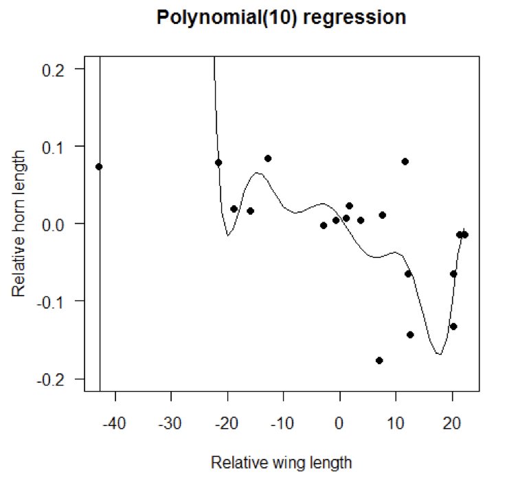 ![Illustration of polynomial regression showing increasing model complexity](../images/ch24/ch24_polynomial_fit.jpeg){#fig-polynomial-fit fig-align="center"} ## Assumptions Multiple regression shares assumptions with simple regression: linearity (in each predictor), independence, normality of residuals, and constant variance. Additionally, predictors should not be perfectly correlated (no perfect multicollinearity). Check assumptions with residual plots. Partial regression plots can help diagnose problems with individual predictors. ## Practical Guidelines Start with a theoretically motivated model rather than throwing in all available predictors. Check for multicollinearity before interpreting coefficients. Use cross-validation to assess prediction performance. Report standardized coefficients when comparing the relative importance of predictors on different scales. Be humble about causation. Multiple regression describes associations; experimental manipulation is needed to establish causation.