Data wrangling is the process of transforming, cleaning, and organizing data to make it suitable for analysis. The dplyr package, part of the tidyverse, provides a powerful and intuitive grammar for data manipulation. This chapter covers the essential tools and techniques for working with data in R.
8.1 The Pipe Operator
One of the most important concepts in modern R programming is the pipe operator. The pipe |> (or the tidyverse’s %>%) passes the result of one operation as the first argument of the next, allowing you to chain operations together in a readable sequence.
Code
# Without pipe: nested and hard to readsummarize(group_by(filter(flights, !is.na(arr_delay)), dest),mean_delay =mean(arr_delay))# With pipe: clear sequence of operationsflights |>filter(!is.na(arr_delay)) |>group_by(dest) |>summarize(mean_delay =mean(arr_delay))
Read the pipe as “then”—take flights, then filter, then group, then summarize. This left-to-right, top-to-bottom flow mirrors how we think about data transformations.
Figure 8.1: The pipe operator passes results from one operation to the next, enabling clear data transformation workflows
8.2 Key dplyr Verbs
The dplyr package provides a grammar for data manipulation centered around five key verbs. These verbs handle most common data manipulation tasks and can be combined to solve complex problems.
filter(): Subset Rows
filter() selects rows that meet specified conditions. This is essential for focusing your analysis on specific subsets of data.
Code
# Load example datalibrary(nycflights13)data(flights)# Flights in November or Decemberflights |>filter(month ==11| month ==12)# Flights with arrival delay greater than 2 hoursflights |>filter(arr_delay >120)# Multiple conditions with ANDflights |>filter(month ==1, day ==1)# Using %in% for set membershipflights |>filter(dest %in%c("SFO", "OAK", "SJC"))
Conditions use comparison operators: - == (equals), != (not equals) - <, >, <=, >= (comparison) - & (and), | (or) - ! (not) - %in% (membership in a set)
select(): Choose Columns
select() picks columns by name, which is useful when working with wide datasets containing many variables.
Code
# Select specific columnsflights |>select(year, month, day)# Select a range of columnsflights |>select(year:day)# Drop columns with minus signflights |>select(-year, -month)# Select by patternflights |>select(starts_with("dep"))flights |>select(ends_with("time"))flights |>select(contains("delay"))# Reorder columnsflights |>select(carrier, flight, everything())
Helper functions for select(): - starts_with(), ends_with(), contains() - match patterns - matches() - regular expressions - num_range() - numeric ranges like “x1”, “x2”, “x3” - everything() - all remaining columns
arrange(): Sort Rows
arrange() reorders rows by column values. By default, it sorts in ascending order.
Code
# Sort by year, then month, then dayflights |>arrange(year, month, day)# Sort in descending orderflights |>arrange(desc(dep_delay))# Missing values always sorted to the endflights |>arrange(dep_time)
mutate(): Create New Columns
mutate() adds new columns that are functions of existing columns. This is one of the most frequently used dplyr functions.
Code
# Create single new columnflights |>mutate(gain = arr_delay - dep_delay)# Create multiple columns, referencing newly created onesflights |>mutate(gain = arr_delay - dep_delay,hours = air_time /60,gain_per_hour = gain / hours )# Keep only new variables with transmute()flights |>transmute(gain = arr_delay - dep_delay,hours = air_time /60,gain_per_hour = gain / hours )
The real power of summarize() emerges when combined with group_by(), which splits data into groups for separate analysis. This is fundamental for comparative statistics.
Code
# Group by destination, then summarizeflights |>group_by(dest) |>summarize(count =n(),mean_delay =mean(arr_delay, na.rm =TRUE),mean_distance =mean(distance) )# Group by multiple variablesflights |>group_by(year, month, day) |>summarize(flights =n(),mean_delay =mean(dep_delay, na.rm =TRUE) )# Grouping affects mutate() tooflights |>group_by(dest) |>mutate(delay_rank =min_rank(desc(arr_delay)),delay_vs_mean = arr_delay -mean(arr_delay, na.rm =TRUE) )
Important notes about grouping: - summarize() removes one level of grouping - Use ungroup() to remove all grouping - Grouped data frames print with group information at the top
Missing values are ubiquitous in real data. In R, missing values are represented as NA (Not Available). Most operations involving NA return NA, which requires careful handling.
Code
# Example of NA behaviorx <-c(1, 2, NA, 4)mean(x) # Returns NAmean(x, na.rm =TRUE) # Returns 2.333333
Detecting Missing Values
Use is.na() to identify missing values:
Code
# Check for NAsis.na(x)# Count missing valuessum(is.na(x))# Count missing values per columnflights |>summarize(across(everything(), ~sum(is.na(.))))
Filtering Missing Values
Code
# Remove rows with NA in specific columnflights |>filter(!is.na(dep_delay))# Keep only complete cases (no NAs in any column)flights |>filter(complete.cases(flights))# Using tidyr's drop_na()flights |>drop_na(dep_delay) # Drop rows with NA in dep_delayflights |>drop_na() # Drop rows with NA in any column
Replacing Missing Values
Code
# Replace NA with specific valueflights |>mutate(dep_delay =replace_na(dep_delay, 0))# Replace NA with meanflights |>mutate(dep_delay =if_else(is.na(dep_delay),mean(dep_delay, na.rm =TRUE), dep_delay))# Using tidyr's replace_na() for multiple columnsflights |>replace_na(list(dep_delay =0, arr_delay =0))
8.5 Joining Data
Real data often comes in multiple tables that need to be combined. Join operations merge tables based on matching values in key columns. Understanding joins is essential for working with relational data.
Different joins handle non-matching rows differently:
Join Type
Function
Result
Left Join
left_join()
Keep all rows from left table, add matching data from right table. Non-matching right rows are dropped, creating NAs in right columns.
Right Join
right_join()
Keep all rows from right table, add matching data from left table. Non-matching left rows are dropped, creating NAs in left columns.
Inner Join
inner_join()
Keep only rows with matches in both tables. Most restrictive join, only complete matches retained.
Full Join
full_join()
Keep all rows from both tables. Creates NAs where matches don’t exist. Most inclusive join.
Semi Join
semi_join()
Keep rows from left table that have matches in right table, but don’t add columns from right. Filtering join.
Anti Join
anti_join()
Keep rows from left table with NO matches in right table. Useful for finding mismatches. Filtering join.
Practical Join Examples
Code
# Inner join: only complete matchesinner_join(measurements, samples, by ="sample_id")# Left join: keep all measurementsleft_join(measurements, samples, by ="sample_id")# Full join: keep everythingfull_join(measurements, samples, by ="sample_id")# Anti join: find measurements without sample info (data quality check)measurements |>anti_join(samples, by ="sample_id")# Semi join: filter samples that have measurementssamples |>semi_join(measurements, by ="sample_id")
Joining on Multiple Keys
Code
# Join on multiple columnstable1 |>left_join(table2, by =c("sample_id", "time_point"))# Join when column names differtable1 |>left_join(table2, by =c("id"="sample_id"))
8.6 Additional dplyr Functions
Beyond the five core verbs, dplyr provides many specialized functions for common data manipulation tasks.
case_when(): Vectorized Conditional Logic
The case_when() function provides a clean way to handle multiple if-else conditions:
The syntax is: condition ~ value. Conditions are evaluated in order, and the first TRUE condition determines the result. Use TRUE ~ value as a catch-all default.
count() and n_distinct()
count() is a convenient shortcut for grouping and counting:
Code
# Count observations per groupflights |>count(carrier)# Equivalent to:flights |>group_by(carrier) |>summarize(n =n())# Count with sortingflights |>count(carrier, sort =TRUE)# Count combinationsflights |>count(carrier, origin)# Add weightsflights |>count(carrier, wt = distance) # sum of distance, not count
While filter() selects rows by condition, slice() and its variants select by position or rank:
Code
# First n rowsflights |>slice_head(n =5)# Last n rowsflights |>slice_tail(n =5)# Random sampleflights |>slice_sample(n =10)flights |>slice_sample(prop =0.01) # 1% of rows# Top n by valueflights |>slice_max(dep_delay, n =5)flights |>slice_min(dep_delay, n =5)# Works with groupsflights |>group_by(carrier) |>slice_max(distance, n =1) # Longest flight per carrier
pull(): Extract a Column as a Vector
select() returns a data frame with one column. pull() extracts a column as a vector:
Code
# Returns a tibble with one columnflights |>select(dep_delay)# Returns a vectorflights |>pull(dep_delay)# Useful for piping into functions that expect vectorsflights |>filter(month ==1) |>pull(dep_delay) |>mean(na.rm =TRUE)
distinct(): Remove Duplicate Rows
Remove duplicate rows based on specified columns:
Code
# Unique values in one columnflights |>distinct(carrier)# Unique combinations of multiple columnsflights |>distinct(carrier, origin)# Keep all columns (removes only exact duplicate rows)flights |>distinct()# Keep other columns along with distinct valuesflights |>distinct(carrier, .keep_all =TRUE)
8.7 Working with Factors
Factors are R’s way of representing categorical data with a fixed set of possible values (called levels). The forcats package (part of tidyverse) provides tools for working with factors, which is essential for controlling category order in analyses and visualizations.
Why Factor Order Matters
By default, R orders factor levels alphabetically, which often produces suboptimal visualizations:
# Original factorstatus <-factor(c("WT", "WT", "KO", "HET", "KO"))# Recode to more descriptive namesstatus_full <-fct_recode(status,"Wild Type"="WT","Knockout"="KO","Heterozygous"="HET")
Collapsing Factor Levels
Combine rare categories using fct_lump_n() or fct_lump_prop():
Code
# Keep only the top 3 most common levelsgene_variants |>mutate(variant =fct_lump_n(variant, n =3))# Combine levels that appear in less than 5% of datagene_variants |>mutate(variant =fct_lump_prop(variant, prop =0.05))# Combine manuallygene_variants |>mutate(variant =fct_collapse(variant,common =c("SNP1", "SNP2", "SNP3"),rare =c("SNP4", "SNP5") ))
8.8 Practice Exercises
Exercise 1: Basic Data Manipulation
Using the nycflights13::flights dataset:
Find all flights that departed in summer (June, July, August)
Select columns related to departure and arrival times
Sort flights by total delay (departure + arrival delay)
Calculate the mean, median, and standard deviation of departure delays by carrier
Find which carrier has the most flights to each destination
Determine the busiest hour of the day (by scheduled departure)
Code
# Part 1: Delay statistics by carrierflights |>group_by(carrier) |>summarize(mean_delay =mean(dep_delay, na.rm =TRUE),median_delay =median(dep_delay, na.rm =TRUE),sd_delay =sd(dep_delay, na.rm =TRUE),n_flights =n() ) |>arrange(desc(mean_delay))# Part 2: Top carrier per destinationflights |>count(dest, carrier) |>group_by(dest) |>slice_max(n, n =1)# Part 3: Busiest departure hourflights |>mutate(hour = dep_time %/%100) |>count(hour, sort =TRUE)
Exercise 3: Data Joining
Create two datasets and practice joining them:
Code
# Create sample datacell_lines <-tibble(cell_line =c("HEK293", "HeLa", "CHO", "Jurkat"),cell_type =c("epithelial", "epithelial", "ovary", "lymphocyte"),species =c("human", "human", "hamster", "human"))experiments <-tibble(cell_line =c("HEK293", "HEK293", "HeLa", "Jurkat", "Jurkat", "PC12"),treatment =c("control", "drug_A", "drug_A", "control", "drug_B", "control"),viability =c(98, 65, 45, 99, 82, 95))# Questions:# 1. Add cell type and species information to experiments# 2. Find cell lines in the database with no experiments# 3. Find experiments for cell lines not in the database# 4. Create a complete dataset with all cell lines and experiments# Solutions:# 1. Left joinexperiments |>left_join(cell_lines, by ="cell_line")# 2. Anti joincell_lines |>anti_join(experiments, by ="cell_line")# 3. Anti join (reverse)experiments |>anti_join(cell_lines, by ="cell_line")# 4. Full joinexperiments |>full_join(cell_lines, by ="cell_line")
Exercise 4: Complex Wrangling Pipeline
Analyze flight delays by time of day and season:
Code
flights |># Create time and season categoriesmutate(time_of_day =case_when( dep_time <600~"night", dep_time <1200~"morning", dep_time <1800~"afternoon",TRUE~"evening" ),season =case_when( month %in%c(12, 1, 2) ~"winter", month %in%c(3, 4, 5) ~"spring", month %in%c(6, 7, 8) ~"summer", month %in%c(9, 10, 11) ~"fall" ) ) |># Remove NAsfilter(!is.na(dep_delay), !is.na(time_of_day)) |># Group and summarizegroup_by(season, time_of_day) |>summarize(mean_delay =mean(dep_delay),median_delay =median(dep_delay),n_flights =n(),.groups ="drop" ) |># Arrange for readabilityarrange(season, time_of_day)
Exercise 5: Working with Factors
Create a publication-ready plot with properly ordered factors:
Code
# Sample biological dataenzyme_data <-tibble(enzyme =rep(c("Lipase", "Amylase", "Protease", "Cellulase"), each =5),temperature =rep(c(20, 30, 40, 50, 60), 4),activity =c(# Lipase12, 24, 48, 36, 18,# Amylase18, 32, 55, 42, 20,# Protease8, 16, 35, 28, 12,# Cellulase15, 28, 62, 48, 22 ))# Calculate optimal temperature for each enzymeoptimal_temps <- enzyme_data |>group_by(enzyme) |>summarize(optimal_temp = temperature[which.max(activity)])# Reorder enzymes by optimal temperatureenzyme_data |>left_join(optimal_temps, by ="enzyme") |>mutate(enzyme =fct_reorder(enzyme, optimal_temp)) |>ggplot(aes(x = temperature, y = activity, color = enzyme)) +geom_line(linewidth =1) +geom_point(size =2) +labs(title ="Enzyme Activity vs Temperature",subtitle ="Ordered by optimal temperature",x ="Temperature (°C)",y ="Enzyme Activity (U/mL)",color ="Enzyme" ) +theme_minimal()
Exercise 6: Missing Data Handling
Practice different strategies for handling missing values:
Code
# Create data with missing valuesmessy_data <-tibble(sample_id =1:10,measurement_1 =c(5.2, NA, 6.8, 7.1, NA, 8.9, 9.2, NA, 7.5, 6.9),measurement_2 =c(12.1, 13.5, NA, 14.2, 15.8, NA, 16.9, 17.2, NA, 14.8),measurement_3 =c(NA, 22.5, 23.1, NA, 24.8, 25.3, NA, 26.7, 27.2, 28.1))# Questions:# 1. How many missing values are in each column?# 2. Remove rows with any missing values# 3. Remove rows with missing values in measurement_1 only# 4. Replace missing values with column means# 5. Flag which measurements are missing# Solutions:# 1. Count NAs per columnmessy_data |>summarize(across(everything(), ~sum(is.na(.))))# 2. Complete cases onlymessy_data |>drop_na()# 3. Drop NAs in specific columnmessy_data |>drop_na(measurement_1)# 4. Replace with meansmessy_data |>mutate(across(starts_with("measurement"),~replace_na(., mean(., na.rm =TRUE))))# 5. Create missing indicatorsmessy_data |>mutate(across(starts_with("measurement"),~is.na(.),.names ="{.col}_missing"))
These exercises cover the core data wrangling operations you’ll use in most analyses. Practice combining these techniques to solve real-world data problems efficiently.
Source Code
# Data Wrangling with dplyr {#sec-data-wrangling}```{r}#| echo: false#| message: falselibrary(tidyverse)theme_set(theme_minimal())```Data wrangling is the process of transforming, cleaning, and organizing data to make it suitable for analysis. The **dplyr** package, part of the tidyverse, provides a powerful and intuitive grammar for data manipulation. This chapter covers the essential tools and techniques for working with data in R.## The Pipe OperatorOne of the most important concepts in modern R programming is the pipe operator. The pipe `|>` (or the tidyverse's `%>%`) passes the result of one operation as the first argument of the next, allowing you to chain operations together in a readable sequence.```{r}#| eval: false# Without pipe: nested and hard to readsummarize(group_by(filter(flights, !is.na(arr_delay)), dest),mean_delay =mean(arr_delay))# With pipe: clear sequence of operationsflights |>filter(!is.na(arr_delay)) |>group_by(dest) |>summarize(mean_delay =mean(arr_delay))```Read the pipe as "then"—take flights, then filter, then group, then summarize. This left-to-right, top-to-bottom flow mirrors how we think about data transformations.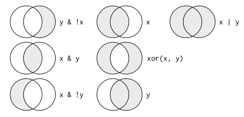{#fig-pipe-operator fig-align="center"}## Key dplyr VerbsThe `dplyr` package provides a grammar for data manipulation centered around five key verbs. These verbs handle most common data manipulation tasks and can be combined to solve complex problems.### filter(): Subset Rows`filter()` selects rows that meet specified conditions. This is essential for focusing your analysis on specific subsets of data.```{r}#| eval: false# Load example datalibrary(nycflights13)data(flights)# Flights in November or Decemberflights |>filter(month ==11| month ==12)# Flights with arrival delay greater than 2 hoursflights |>filter(arr_delay >120)# Multiple conditions with ANDflights |>filter(month ==1, day ==1)# Using %in% for set membershipflights |>filter(dest %in%c("SFO", "OAK", "SJC"))```Conditions use comparison operators:- `==` (equals), `!=` (not equals)- `<`, `>`, `<=`, `>=` (comparison)- `&` (and), `|` (or)- `!` (not)- `%in%` (membership in a set)### select(): Choose Columns`select()` picks columns by name, which is useful when working with wide datasets containing many variables.```{r}#| eval: false# Select specific columnsflights |>select(year, month, day)# Select a range of columnsflights |>select(year:day)# Drop columns with minus signflights |>select(-year, -month)# Select by patternflights |>select(starts_with("dep"))flights |>select(ends_with("time"))flights |>select(contains("delay"))# Reorder columnsflights |>select(carrier, flight, everything())```Helper functions for `select()`:- `starts_with()`, `ends_with()`, `contains()` - match patterns- `matches()` - regular expressions- `num_range()` - numeric ranges like "x1", "x2", "x3"- `everything()` - all remaining columns### arrange(): Sort Rows`arrange()` reorders rows by column values. By default, it sorts in ascending order.```{r}#| eval: false# Sort by year, then month, then dayflights |>arrange(year, month, day)# Sort in descending orderflights |>arrange(desc(dep_delay))# Missing values always sorted to the endflights |>arrange(dep_time)```### mutate(): Create New Columns`mutate()` adds new columns that are functions of existing columns. This is one of the most frequently used dplyr functions.```{r}#| eval: false# Create single new columnflights |>mutate(gain = arr_delay - dep_delay)# Create multiple columns, referencing newly created onesflights |>mutate(gain = arr_delay - dep_delay,hours = air_time /60,gain_per_hour = gain / hours )# Keep only new variables with transmute()flights |>transmute(gain = arr_delay - dep_delay,hours = air_time /60,gain_per_hour = gain / hours )```Common functions used with `mutate()`:- Arithmetic: `+`, `-`, `*`, `/`, `^`- Modular arithmetic: `%/%` (integer division), `%%` (remainder)- Logs: `log()`, `log2()`, `log10()`- Offsets: `lead()`, `lag()`- Cumulative: `cumsum()`, `cumprod()`, `cummin()`, `cummax()`- Ranking: `min_rank()`, `row_number()`, `dense_rank()`### summarize(): Aggregate Data`summarize()` (or `summarise()`) collapses multiple rows into summary values. It's particularly powerful when combined with `group_by()`.```{r}#| eval: false# Single summary statisticflights |>summarize(mean_delay =mean(dep_delay, na.rm =TRUE))# Multiple summary statisticsflights |>summarize(mean_delay =mean(dep_delay, na.rm =TRUE),median_delay =median(dep_delay, na.rm =TRUE),sd_delay =sd(dep_delay, na.rm =TRUE),n =n() )```Common summary functions:- Central tendency: `mean()`, `median()`- Spread: `sd()`, `var()`, `IQR()`, `mad()`- Range: `min()`, `max()`, `quantile()`- Position: `first()`, `last()`, `nth()`- Count: `n()`, `n_distinct()`## Grouping with group_by()The real power of `summarize()` emerges when combined with `group_by()`, which splits data into groups for separate analysis. This is fundamental for comparative statistics.```{r}#| eval: false# Group by destination, then summarizeflights |>group_by(dest) |>summarize(count =n(),mean_delay =mean(arr_delay, na.rm =TRUE),mean_distance =mean(distance) )# Group by multiple variablesflights |>group_by(year, month, day) |>summarize(flights =n(),mean_delay =mean(dep_delay, na.rm =TRUE) )# Grouping affects mutate() tooflights |>group_by(dest) |>mutate(delay_rank =min_rank(desc(arr_delay)),delay_vs_mean = arr_delay -mean(arr_delay, na.rm =TRUE) )```Important notes about grouping:- `summarize()` removes one level of grouping- Use `ungroup()` to remove all grouping- Grouped data frames print with group information at the top```{r}#| eval: false# Remove groupingflights |>group_by(dest) |>summarize(mean_delay =mean(arr_delay, na.rm =TRUE)) |>ungroup()```## Handling Missing ValuesMissing values are ubiquitous in real data. In R, missing values are represented as `NA` (Not Available). Most operations involving `NA` return `NA`, which requires careful handling.```{r}#| eval: false# Example of NA behaviorx <-c(1, 2, NA, 4)mean(x) # Returns NAmean(x, na.rm =TRUE) # Returns 2.333333```### Detecting Missing ValuesUse `is.na()` to identify missing values:```{r}#| eval: false# Check for NAsis.na(x)# Count missing valuessum(is.na(x))# Count missing values per columnflights |>summarize(across(everything(), ~sum(is.na(.))))```### Filtering Missing Values```{r}#| eval: false# Remove rows with NA in specific columnflights |>filter(!is.na(dep_delay))# Keep only complete cases (no NAs in any column)flights |>filter(complete.cases(flights))# Using tidyr's drop_na()flights |>drop_na(dep_delay) # Drop rows with NA in dep_delayflights |>drop_na() # Drop rows with NA in any column```### Replacing Missing Values```{r}#| eval: false# Replace NA with specific valueflights |>mutate(dep_delay =replace_na(dep_delay, 0))# Replace NA with meanflights |>mutate(dep_delay =if_else(is.na(dep_delay),mean(dep_delay, na.rm =TRUE), dep_delay))# Using tidyr's replace_na() for multiple columnsflights |>replace_na(list(dep_delay =0, arr_delay =0))```## Joining DataReal data often comes in multiple tables that need to be combined. Join operations merge tables based on matching values in key columns. Understanding joins is essential for working with relational data.### Basic Join Example```{r}#| eval: false# Example tablessamples <-tibble(sample_id =c("S1", "S2", "S3"),treatment =c("control", "low", "high"),concentration =c(0.0, 0.1, 1.0))measurements <-tibble(sample_id =c("S1", "S1", "S2", "S2", "S3", "S3"),replicate =c(1, 2, 1, 2, 1, 2),value =c(2.3, 2.1, 5.4, 5.6, 10.2, 10.8))# Join tablesmeasurements |>left_join(samples, by ="sample_id")```### Types of JoinsDifferent joins handle non-matching rows differently:| Join Type | Function | Result ||:----------|:---------|:-------|| **Left Join** |`left_join()`| Keep all rows from left table, add matching data from right table. Non-matching right rows are dropped, creating NAs in right columns. || **Right Join** |`right_join()`| Keep all rows from right table, add matching data from left table. Non-matching left rows are dropped, creating NAs in left columns. || **Inner Join** |`inner_join()`| Keep only rows with matches in both tables. Most restrictive join, only complete matches retained. || **Full Join** |`full_join()`| Keep all rows from both tables. Creates NAs where matches don't exist. Most inclusive join. || **Semi Join** |`semi_join()`| Keep rows from left table that have matches in right table, but don't add columns from right. Filtering join. || **Anti Join** |`anti_join()`| Keep rows from left table with NO matches in right table. Useful for finding mismatches. Filtering join. |### Practical Join Examples```{r}#| eval: false# Inner join: only complete matchesinner_join(measurements, samples, by ="sample_id")# Left join: keep all measurementsleft_join(measurements, samples, by ="sample_id")# Full join: keep everythingfull_join(measurements, samples, by ="sample_id")# Anti join: find measurements without sample info (data quality check)measurements |>anti_join(samples, by ="sample_id")# Semi join: filter samples that have measurementssamples |>semi_join(measurements, by ="sample_id")```### Joining on Multiple Keys```{r}#| eval: false# Join on multiple columnstable1 |>left_join(table2, by =c("sample_id", "time_point"))# Join when column names differtable1 |>left_join(table2, by =c("id"="sample_id"))```## Additional dplyr FunctionsBeyond the five core verbs, dplyr provides many specialized functions for common data manipulation tasks.### case_when(): Vectorized Conditional LogicThe `case_when()` function provides a clean way to handle multiple if-else conditions:```{r}#| eval: false# Create sample dataexpression_data <-tibble(gene =c("BRCA1", "TP53", "EGFR", "KRAS", "MYC"),fold_change =c(0.5, 1.2, 3.5, -2.1, 0.9))# Classify regulation statusexpression_data |>mutate(regulation =case_when( fold_change >2~"strongly upregulated", fold_change >1~"upregulated", fold_change <-2~"strongly downregulated", fold_change <-1~"downregulated",TRUE~"unchanged"# default case ) )```The syntax is: `condition ~ value`. Conditions are evaluated in order, and the first TRUE condition determines the result. Use `TRUE ~ value` as a catch-all default.### count() and n_distinct()`count()` is a convenient shortcut for grouping and counting:```{r}#| eval: false# Count observations per groupflights |>count(carrier)# Equivalent to:flights |>group_by(carrier) |>summarize(n =n())# Count with sortingflights |>count(carrier, sort =TRUE)# Count combinationsflights |>count(carrier, origin)# Add weightsflights |>count(carrier, wt = distance) # sum of distance, not count```Use `n_distinct()` to count unique values:```{r}#| eval: false# Count unique destinations per carrierflights |>group_by(carrier) |>summarize(n_flights =n(),n_destinations =n_distinct(dest) )```### slice() Variants: Select Rows by PositionWhile `filter()` selects rows by condition, `slice()` and its variants select by position or rank:```{r}#| eval: false# First n rowsflights |>slice_head(n =5)# Last n rowsflights |>slice_tail(n =5)# Random sampleflights |>slice_sample(n =10)flights |>slice_sample(prop =0.01) # 1% of rows# Top n by valueflights |>slice_max(dep_delay, n =5)flights |>slice_min(dep_delay, n =5)# Works with groupsflights |>group_by(carrier) |>slice_max(distance, n =1) # Longest flight per carrier```### pull(): Extract a Column as a Vector`select()` returns a data frame with one column. `pull()` extracts a column as a vector:```{r}#| eval: false# Returns a tibble with one columnflights |>select(dep_delay)# Returns a vectorflights |>pull(dep_delay)# Useful for piping into functions that expect vectorsflights |>filter(month ==1) |>pull(dep_delay) |>mean(na.rm =TRUE)```### distinct(): Remove Duplicate RowsRemove duplicate rows based on specified columns:```{r}#| eval: false# Unique values in one columnflights |>distinct(carrier)# Unique combinations of multiple columnsflights |>distinct(carrier, origin)# Keep all columns (removes only exact duplicate rows)flights |>distinct()# Keep other columns along with distinct valuesflights |>distinct(carrier, .keep_all =TRUE)```## Working with FactorsFactors are R's way of representing categorical data with a fixed set of possible values (called levels). The **forcats** package (part of tidyverse) provides tools for working with factors, which is essential for controlling category order in analyses and visualizations.### Why Factor Order MattersBy default, R orders factor levels alphabetically, which often produces suboptimal visualizations:```{r}#| label: fig-gene-alphabetical#| fig-cap: "Gene expression in default alphabetical order makes comparison difficult"#| fig-width: 6#| fig-height: 4#| eval: false# Sample datagene_data <-tibble(gene =c("BRCA1", "TP53", "EGFR", "KRAS", "MYC"),expression =c(5.2, 8.1, 3.4, 6.7, 9.2))# Default: alphabetical orderggplot(gene_data, aes(x = gene, y = expression)) +geom_col(fill ="steelblue") +labs(title ="Gene Expression (Alphabetical Order)",x ="Gene",y ="Expression Level" ) +theme_minimal()```### Reordering FactorsUse `fct_reorder()` to order factors by another variable:```{r}#| label: fig-gene-ordered#| fig-cap: "Gene expression ordered by value facilitates easy comparison and pattern recognition"#| fig-width: 6#| fig-height: 4#| eval: false# Reorder by expression valuelibrary(forcats)gene_data |>mutate(gene =fct_reorder(gene, expression)) |>ggplot(aes(x = gene, y = expression)) +geom_col(fill ="steelblue") +labs(title ="Gene Expression (Ordered by Value)",x ="Gene",y ="Expression Level" ) +theme_minimal()```### Additional forcats Functions```{r}#| eval: false# Reorder by frequencygene_counts |>mutate(gene =fct_infreq(gene))# Reverse factor ordergene_data |>mutate(gene =fct_rev(gene))# Reorder manuallygene_data |>mutate(gene =fct_relevel(gene, "TP53", "MYC", "BRCA1"))```### Recoding Factor LevelsUse `fct_recode()` to change level names:```{r}#| eval: false# Original factorstatus <-factor(c("WT", "WT", "KO", "HET", "KO"))# Recode to more descriptive namesstatus_full <-fct_recode(status,"Wild Type"="WT","Knockout"="KO","Heterozygous"="HET")```### Collapsing Factor LevelsCombine rare categories using `fct_lump_n()` or `fct_lump_prop()`:```{r}#| eval: false# Keep only the top 3 most common levelsgene_variants |>mutate(variant =fct_lump_n(variant, n =3))# Combine levels that appear in less than 5% of datagene_variants |>mutate(variant =fct_lump_prop(variant, prop =0.05))# Combine manuallygene_variants |>mutate(variant =fct_collapse(variant,common =c("SNP1", "SNP2", "SNP3"),rare =c("SNP4", "SNP5") ))```## Practice Exercises::: {.callout-note}### Exercise 1: Basic Data ManipulationUsing the `nycflights13::flights` dataset:1. Find all flights that departed in summer (June, July, August)2. Select columns related to departure and arrival times3. Sort flights by total delay (departure + arrival delay)4. Create a new variable for flight speed in mph```{r}#| eval: falselibrary(nycflights13)# Your solution hereflights |>filter(month %in%c(6, 7, 8)) |>select(month, day, dep_time, arr_time, dep_delay, arr_delay) |>mutate(total_delay = dep_delay + arr_delay,speed_mph = distance / (air_time /60) ) |>arrange(desc(total_delay))```:::::: {.callout-note}### Exercise 2: Grouping and Summarizing1. Calculate the mean, median, and standard deviation of departure delays by carrier2. Find which carrier has the most flights to each destination3. Determine the busiest hour of the day (by scheduled departure)```{r}#| eval: false# Part 1: Delay statistics by carrierflights |>group_by(carrier) |>summarize(mean_delay =mean(dep_delay, na.rm =TRUE),median_delay =median(dep_delay, na.rm =TRUE),sd_delay =sd(dep_delay, na.rm =TRUE),n_flights =n() ) |>arrange(desc(mean_delay))# Part 2: Top carrier per destinationflights |>count(dest, carrier) |>group_by(dest) |>slice_max(n, n =1)# Part 3: Busiest departure hourflights |>mutate(hour = dep_time %/%100) |>count(hour, sort =TRUE)```:::::: {.callout-note}### Exercise 3: Data JoiningCreate two datasets and practice joining them:```{r}#| eval: false# Create sample datacell_lines <-tibble(cell_line =c("HEK293", "HeLa", "CHO", "Jurkat"),cell_type =c("epithelial", "epithelial", "ovary", "lymphocyte"),species =c("human", "human", "hamster", "human"))experiments <-tibble(cell_line =c("HEK293", "HEK293", "HeLa", "Jurkat", "Jurkat", "PC12"),treatment =c("control", "drug_A", "drug_A", "control", "drug_B", "control"),viability =c(98, 65, 45, 99, 82, 95))# Questions:# 1. Add cell type and species information to experiments# 2. Find cell lines in the database with no experiments# 3. Find experiments for cell lines not in the database# 4. Create a complete dataset with all cell lines and experiments# Solutions:# 1. Left joinexperiments |>left_join(cell_lines, by ="cell_line")# 2. Anti joincell_lines |>anti_join(experiments, by ="cell_line")# 3. Anti join (reverse)experiments |>anti_join(cell_lines, by ="cell_line")# 4. Full joinexperiments |>full_join(cell_lines, by ="cell_line")```:::::: {.callout-note}### Exercise 4: Complex Wrangling PipelineAnalyze flight delays by time of day and season:```{r}#| eval: falseflights |># Create time and season categoriesmutate(time_of_day =case_when( dep_time <600~"night", dep_time <1200~"morning", dep_time <1800~"afternoon",TRUE~"evening" ),season =case_when( month %in%c(12, 1, 2) ~"winter", month %in%c(3, 4, 5) ~"spring", month %in%c(6, 7, 8) ~"summer", month %in%c(9, 10, 11) ~"fall" ) ) |># Remove NAsfilter(!is.na(dep_delay), !is.na(time_of_day)) |># Group and summarizegroup_by(season, time_of_day) |>summarize(mean_delay =mean(dep_delay),median_delay =median(dep_delay),n_flights =n(),.groups ="drop" ) |># Arrange for readabilityarrange(season, time_of_day)```:::::: {.callout-note}### Exercise 5: Working with FactorsCreate a publication-ready plot with properly ordered factors:```{r}#| eval: false# Sample biological dataenzyme_data <-tibble(enzyme =rep(c("Lipase", "Amylase", "Protease", "Cellulase"), each =5),temperature =rep(c(20, 30, 40, 50, 60), 4),activity =c(# Lipase12, 24, 48, 36, 18,# Amylase18, 32, 55, 42, 20,# Protease8, 16, 35, 28, 12,# Cellulase15, 28, 62, 48, 22 ))# Calculate optimal temperature for each enzymeoptimal_temps <- enzyme_data |>group_by(enzyme) |>summarize(optimal_temp = temperature[which.max(activity)])# Reorder enzymes by optimal temperatureenzyme_data |>left_join(optimal_temps, by ="enzyme") |>mutate(enzyme =fct_reorder(enzyme, optimal_temp)) |>ggplot(aes(x = temperature, y = activity, color = enzyme)) +geom_line(linewidth =1) +geom_point(size =2) +labs(title ="Enzyme Activity vs Temperature",subtitle ="Ordered by optimal temperature",x ="Temperature (°C)",y ="Enzyme Activity (U/mL)",color ="Enzyme" ) +theme_minimal()```:::::: {.callout-note}### Exercise 6: Missing Data HandlingPractice different strategies for handling missing values:```{r}#| eval: false# Create data with missing valuesmessy_data <-tibble(sample_id =1:10,measurement_1 =c(5.2, NA, 6.8, 7.1, NA, 8.9, 9.2, NA, 7.5, 6.9),measurement_2 =c(12.1, 13.5, NA, 14.2, 15.8, NA, 16.9, 17.2, NA, 14.8),measurement_3 =c(NA, 22.5, 23.1, NA, 24.8, 25.3, NA, 26.7, 27.2, 28.1))# Questions:# 1. How many missing values are in each column?# 2. Remove rows with any missing values# 3. Remove rows with missing values in measurement_1 only# 4. Replace missing values with column means# 5. Flag which measurements are missing# Solutions:# 1. Count NAs per columnmessy_data |>summarize(across(everything(), ~sum(is.na(.))))# 2. Complete cases onlymessy_data |>drop_na()# 3. Drop NAs in specific columnmessy_data |>drop_na(measurement_1)# 4. Replace with meansmessy_data |>mutate(across(starts_with("measurement"),~replace_na(., mean(., na.rm =TRUE))))# 5. Create missing indicatorsmessy_data |>mutate(across(starts_with("measurement"),~is.na(.),.names ="{.col}_missing"))```:::These exercises cover the core data wrangling operations you'll use in most analyses. Practice combining these techniques to solve real-world data problems efficiently.
