One of the most common questions in data analysis is whether two groups differ. Is the mean expression level different between treatment and control? Does the new material have different strength than the standard? Do patients on drug A have different outcomes than patients on drug B?
The t-test is the classic method for comparing means. It compares the observed difference between groups to the variability expected by chance, producing a test statistic that follows a t-distribution under the null hypothesis of no difference.
17.2 The T-Distribution
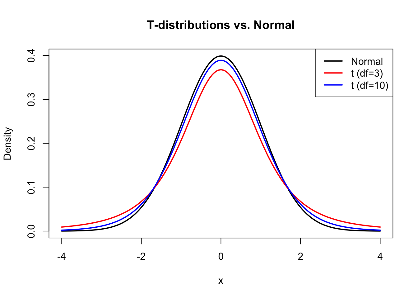
The t-distribution, introduced by William Sealy Gosset writing under the pseudonym “Student” (Student 1908), resembles the normal distribution but has heavier tails. This accounts for the extra uncertainty that comes from estimating the population standard deviation from sample data.
The t-distribution is characterized by its degrees of freedom (df). As df increases, the t-distribution approaches the normal distribution. For small samples, the heavier tails mean that extreme values are more likely, leading to wider confidence intervals and more conservative tests.
Code
# Compare t-distributions with different dfx <-seq(-4, 4, length.out =200)plot(x, dnorm(x), type ="l", lwd =2, col ="black",xlab ="x", ylab ="Density",main ="T-distributions vs. Normal")lines(x, dt(x, df =3), lwd =2, col ="red")lines(x, dt(x, df =10), lwd =2, col ="blue")legend("topright",legend =c("Normal", "t (df=3)", "t (df=10)"),col =c("black", "red", "blue"), lwd =2)
Figure 17.1: The t-distribution has heavier tails than the normal, especially with low degrees of freedom
Why Heavier Tails Matter in Practice
The heavier tails of the t-distribution have real practical consequences. When you estimate the standard deviation from a small sample, you might underestimate or overestimate the true value. The t-distribution accounts for this uncertainty by assigning more probability to extreme values.
Consider this concrete example: suppose you’re estimating voter support from a poll of 25 likely voters. With the true population proportion unknown and estimated from the sample, how wide should your confidence interval be?
Code
# Demonstrate the practical difference between normal and t-based intervalsset.seed(2016)# Simulate: true support is 48.5%, poll 25 peopletrue_support <-0.485n_poll <-25# One poll resultpoll_result <-rbinom(1, n_poll, true_support) / n_pollpoll_se <-sqrt(poll_result * (1- poll_result) / n_poll)# Compare critical valuesz_crit <-qnorm(0.975) # Normal: 1.96t_crit <-qt(0.975, df = n_poll -1) # t with 24 df: 2.06# Calculate intervalsnormal_ci <-c(poll_result - z_crit * poll_se, poll_result + z_crit * poll_se)t_ci <-c(poll_result - t_crit * poll_se, poll_result + t_crit * poll_se)cat("Poll result:", round(poll_result *100, 1), "%\n")
With only 25 observations, the t-distribution gives a critical value of about 2.06 instead of 1.96. This ~5% wider interval provides better coverage when the sample standard deviation might deviate substantially from the population value.
The difference matters most in the tails. For extreme values (like being 2.5+ standard errors away from the mean), the t-distribution assigns noticeably more probability:
Code
# Probability of being more than 2.5 SE from the meanprob_extreme_normal <-2*pnorm(-2.5)prob_extreme_t <-2*pt(-2.5, df =24)cat("P(|Z| > 2.5) with normal distribution:", round(prob_extreme_normal, 4), "\n")
P(|Z| > 2.5) with normal distribution: 0.0124
Code
cat("P(|T| > 2.5) with t(df=24):", round(prob_extreme_t, 4), "\n")
P(|T| > 2.5) with t(df=24): 0.0197
Code
cat("The t-distribution gives", round(prob_extreme_t/prob_extreme_normal, 1),"times higher probability to extreme values\n")
The t-distribution gives 1.6 times higher probability to extreme values
This is why using the normal distribution instead of the t-distribution for small samples leads to confidence intervals that are too narrow and p-values that are too small—both resulting in overconfident conclusions.
17.3 One-Sample T-Test
The one-sample t-test compares a sample mean to a hypothesized population value. The null hypothesis is that the population mean equals the specified value: \(H_0: \mu = \mu_0\).
The test statistic is:
\[t = \frac{\bar{x} - \mu_0}{s / \sqrt{n}}\]
This is the difference between the sample mean and hypothesized value, divided by the standard error of the mean. Under the null hypothesis, this statistic follows a t-distribution with \(n-1\) degrees of freedom.
Code
# One-sample t-test example# Does this sample come from a population with mean = 100?set.seed(42)sample_data <-rnorm(25, mean =105, sd =15)t.test(sample_data, mu =100)
    One Sample t-test

data:  sample_data
t = 1.9936, df = 24, p-value = 0.05768
alternative hypothesis: true mean is not equal to 100
95 percent confidence interval:
  99.72443 115.90166
sample estimates:
mean of x
  107.813
The output shows the t-statistic, degrees of freedom, p-value, confidence interval, and sample mean. The small p-value indicates evidence that the true mean differs from 100.
17.4 Two-Sample T-Test
The two-sample (independent samples) t-test compares means from two independent groups. The null hypothesis is that the population means are equal: \(H_0: \mu_1 = \mu_2\).
The test assumes: - Independence of observations within and between groups - Normally distributed populations (or large samples) - Equal variances in both groups (for the standard version)
Code
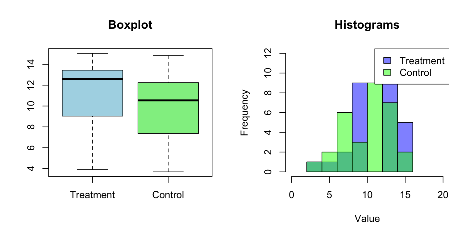
# Two-sample t-test exampleset.seed(518)treatment <-rnorm(n =30, mean =12, sd =3)control <-rnorm(n =30, mean =10, sd =3)# Visualize the datapar(mfrow =c(1, 2))boxplot(treatment, control, names =c("Treatment", "Control"),col =c("lightblue", "lightgreen"), main ="Boxplot")# Combined histogramhist(treatment, col =rgb(0, 0, 1, 0.5), xlim =c(0, 20),main ="Histograms", xlab ="Value")hist(control, col =rgb(0, 1, 0, 0.5), add =TRUE)legend("topright", legend =c("Treatment", "Control"),fill =c(rgb(0, 0, 1, 0.5), rgb(0, 1, 0, 0.5)))
Figure 17.2: Visualization of two groups before performing a two-sample t-test
Code
# Perform the t-testt.test(treatment, control)
    Welch Two Sample t-test

data:  treatment and control
t = 1.3224, df = 57.98, p-value = 0.1912
alternative hypothesis: true difference in means is not equal to 0
95 percent confidence interval:
 -0.5256045  2.5718411
sample estimates:
mean of x mean of y
 11.08437  10.06125
17.5 Welch’s T-Test
The classic two-sample t-test assumes equal variances. When this assumption is violated, Welch’s t-test provides a better alternative. It adjusts the degrees of freedom to account for unequal variances.
R’s t.test() function uses Welch’s test by default. To use the equal-variance version, set var.equal = TRUE.
Code
# When variances are unequalset.seed(42)group1 <-rnorm(30, mean =50, sd =5)group2 <-rnorm(30, mean =52, sd =15)# Welch's test (default)t.test(group1, group2)
    Welch Two Sample t-test

data:  group1 and group2
t = 0.055423, df = 37.98, p-value = 0.9561
alternative hypothesis: true difference in means is not equal to 0
95 percent confidence interval:
 -6.095093  6.438216
sample estimates:
mean of x mean of y
 50.34293  50.17137
    Two Sample t-test

data:  group1 and group2
t = 0.055423, df = 58, p-value = 0.956
alternative hypothesis: true difference in means is not equal to 0
95 percent confidence interval:
 -6.024786  6.367910
sample estimates:
mean of x mean of y
 50.34293  50.17137
17.6 Paired T-Test
When observations in two groups are naturally paired—the same subjects measured twice, matched pairs, or before-and-after measurements—the paired t-test is more appropriate. It tests whether the mean difference within pairs is zero.
The paired t-test is more powerful than the two-sample test when pairs are positively correlated, because it removes between-subject variability.
Code
# Paired t-test example: before and after treatmentset.seed(123)n <-20before <-rnorm(n, mean =100, sd =15)# After measurements are correlated with beforeafter <- before +rnorm(n, mean =5, sd =5)# Paired test (correct for this data)t.test(after, before, paired =TRUE)
    Paired t-test

data:  after and before
t = 5.1123, df = 19, p-value = 6.19e-05
alternative hypothesis: true mean difference is not equal to 0
95 percent confidence interval:
 2.801598 6.685830
sample estimates:
mean difference
       4.743714
Code
# Compare to unpaired (less power)t.test(after, before, paired =FALSE)
    Welch Two Sample t-test

data:  after and before
t = 1.0209, df = 37.992, p-value = 0.3138
alternative hypothesis: true difference in means is not equal to 0
95 percent confidence interval:
 -4.663231 14.150660
sample estimates:
mean of x mean of y
 106.8681  102.1244
Notice that the paired test produces a smaller p-value because it accounts for the correlation between measurements on the same subject.
17.7 One-Tailed vs. Two-Tailed Tests
By default, t.test() performs a two-tailed test. For a one-tailed test, specify the alternative hypothesis:
Code
# Two-tailed (default): H_A: treatment ≠ controlt.test(treatment, control, alternative ="two.sided")$p.value
[1] 0.1912327
Code
# One-tailed: H_A: treatment > controlt.test(treatment, control, alternative ="greater")$p.value
[1] 0.09561633
Code
# One-tailed: H_A: treatment < controlt.test(treatment, control, alternative ="less")$p.value
[1] 0.9043837
Use one-tailed tests only when you have a strong prior reason to expect an effect in a specific direction and would not act on an effect in the opposite direction.
17.8 Checking Assumptions
T-tests assume normally distributed data (or large samples) and, for the standard two-sample test, equal variances. Check these assumptions before interpreting results.
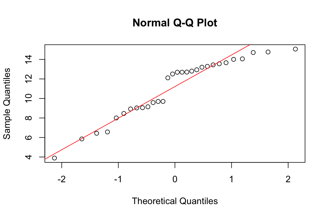
Normality: Use histograms, Q-Q plots, or formal tests like Shapiro-Wilk.
Code
# Check normality with Q-Q plotqqnorm(treatment)qqline(treatment, col ="red")
Figure 17.3: Q-Q plot for assessing normality: points following the line suggest approximate normality
Code
# Shapiro-Wilk test for normalityshapiro.test(treatment)
    Shapiro-Wilk normality test

data:  treatment
W = 0.9115, p-value = 0.01624
A non-significant Shapiro-Wilk test suggests the data are consistent with normality. However, this test has low power for small samples and may reject normality for trivial deviations with large samples.
Equal variances: Compare standard deviations or use Levene’s test.
Code
# Compare standard deviationssd(treatment)
[1] 3.024138
Code
sd(control)
[1] 2.968592
Code
# Levene's test (from car package)# car::leveneTest(c(treatment, control), # factor(rep(c("treatment", "control"), each = 30)))
17.9 Effect Size: Cohen’s d
Statistical significance does not tell you how large an effect is. Cohen’s d measures effect size as the standardized difference between means:
\[d = \frac{\bar{x}_1 - \bar{x}_2}{s_{pooled}}\]
where \(s_{pooled}\) is the pooled standard deviation.
Conventional interpretations: \(|d| = 0.2\) is small, \(|d| = 0.5\) is medium, \(|d| = 0.8\) is large. However, context matters—a small d might be practically important in some fields.
    Welch Two Sample t-test

data:  drug and placebo
t = 1.2147, df = 75.923, p-value = 0.2282
alternative hypothesis: true difference in means is not equal to 0
95 percent confidence interval:
 -1.990367  8.213525
sample estimates:
mean of x mean of y
 72.26982  69.15824
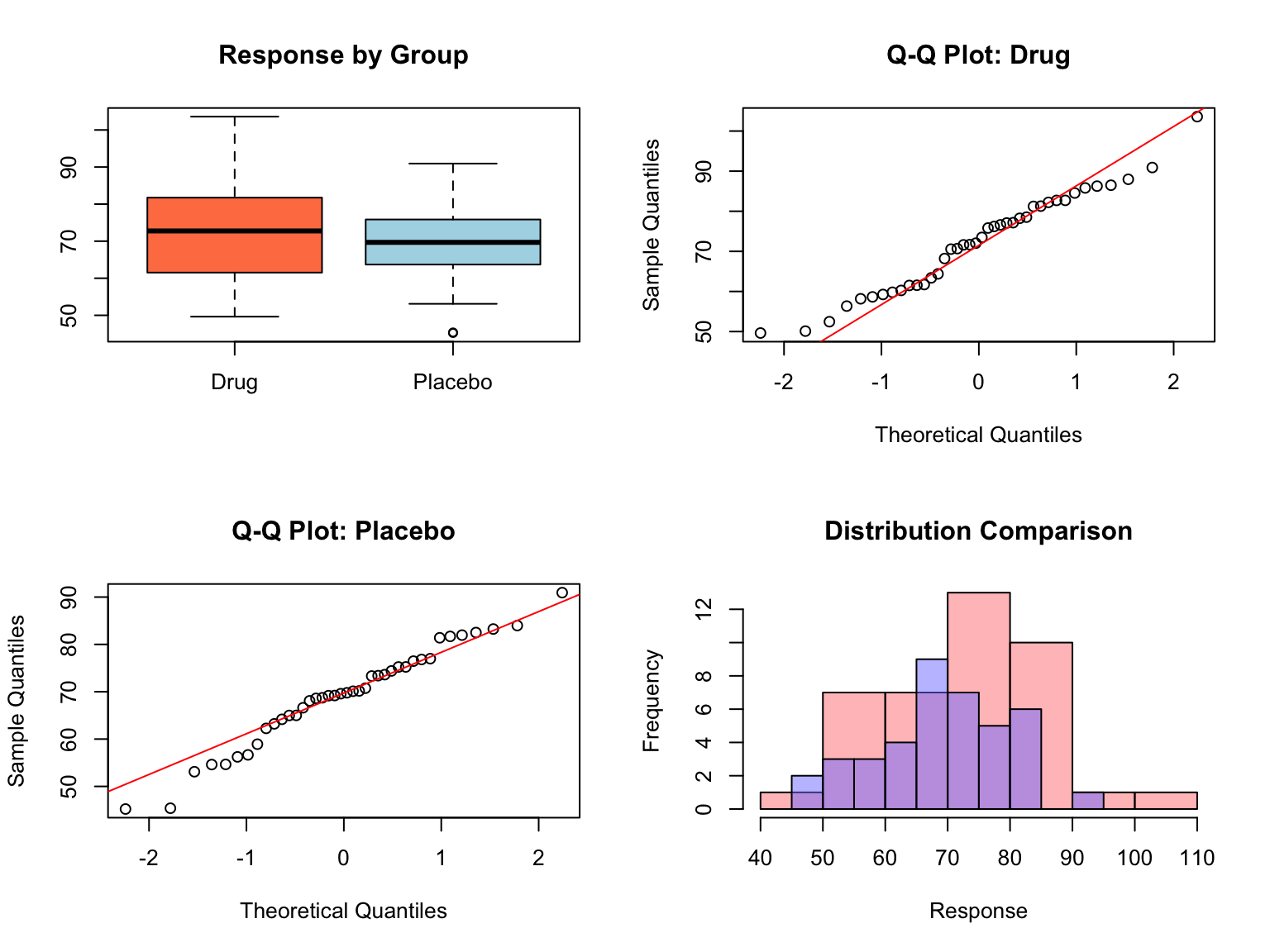
The t-test shows a significant difference (p < 0.05), and Cohen’s d indicates a medium effect size. We can conclude that the drug group shows higher response than the placebo group, with the mean difference being about 0.4 standard deviations.
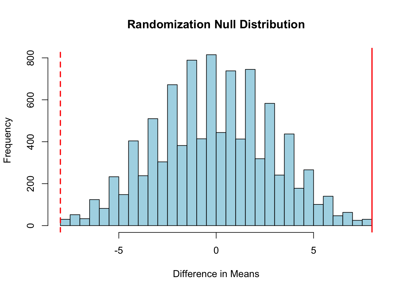
17.11 Randomization Tests as an Alternative
When normality assumptions are questionable and sample sizes are small, randomization (permutation) tests provide a non-parametric alternative to the t-test. The logic is elegant: if there is no difference between groups, then the group labels are arbitrary and could be shuffled without affecting the distribution of the test statistic.
Code
# Randomization test exampleset.seed(42)group_A <-c(23, 25, 28, 31, 35, 29)group_B <-c(18, 20, 22, 19, 21, 23)# Observed differenceobs_diff <-mean(group_A) -mean(group_B)# Combine all observationsall_data <-c(group_A, group_B)n_A <-length(group_A)n_B <-length(group_B)# Generate null distribution by permutationn_perms <-10000perm_diffs <-numeric(n_perms)for (i in1:n_perms) { shuffled <-sample(all_data) perm_diffs[i] <-mean(shuffled[1:n_A]) -mean(shuffled[(n_A+1):(n_A+n_B)])}# Plot null distributionhist(perm_diffs, breaks =50, col ="lightblue",main ="Randomization Null Distribution",xlab ="Difference in Means")abline(v = obs_diff, col ="red", lwd =2)abline(v =-obs_diff, col ="red", lwd =2, lty =2)# Two-tailed p-valuep_value <-mean(abs(perm_diffs) >=abs(obs_diff))cat("Observed difference:", round(obs_diff, 2), "\n")
Observed difference: 8
Code
cat("Permutation p-value:", p_value, "\n")
Permutation p-value: 0.0039
Figure 17.5: Permutation test null distribution with observed difference (red line) for comparison
The randomization test makes no assumptions about the underlying distribution—it only assumes that observations are exchangeable under the null hypothesis. This makes it robust to non-normality and outliers.
When to Use Randomization Tests
Sample sizes are small (n < 20 per group)
Data are clearly non-normal or contain outliers
You want to avoid distributional assumptions
As a sensitivity analysis to complement parametric results
17.12 Choosing the Right T-Test
Scenario
Test
R Function
Compare sample mean to known value
One-sample
t.test(x, mu = value)
Compare two independent groups
Two-sample (Welch’s)
t.test(x, y)
Compare two independent groups (equal variance)
Two-sample (Student’s)
t.test(x, y, var.equal = TRUE)
Compare paired measurements
Paired
t.test(x, y, paired = TRUE)
Decision guidelines:
If comparing to a fixed, known value: one-sample t-test
If observations in groups are naturally paired: paired t-test
If groups are independent with potentially unequal variances: Welch’s t-test (the default)
If groups are independent and you have strong evidence of equal variances: Student’s t-test
When in doubt, use Welch’s t-test—it performs nearly as well as Student’s t-test when variances are equal and much better when they are not.
17.13 Summary
The t-test family provides essential tools for comparing means:
One-sample tests compare a sample to a hypothesized value
Two-sample tests compare independent groups
Paired tests compare matched or repeated measurements
Welch’s version handles unequal variances (recommended default)
Randomization tests provide a distribution-free alternative
Always visualize your data, check assumptions, and report effect sizes alongside p-values. A statistically significant result is only meaningful if the underlying assumptions are reasonable and the effect size is practically relevant.
17.14 Practice Exercises
Exercise H.1: One-Sample t-test
Generate a sample of 30 observations from a normal distribution with mean 105 and SD 15
Test whether the mean differs significantly from 100
Interpret the p-value and confidence interval
What happens to the p-value when you increase the sample size?
Code
set.seed(42)sample_data <-rnorm(30, mean =105, sd =15)t.test(sample_data, mu =100)
Exercise H.2: Two-Sample t-test
Create a dummy dataset with one continuous and one categorical variable:
Draw samples of 100 observations from two normal distributions with slightly different means but equal standard deviations
Perform a two-sample t-test
Visualize the data with a boxplot
Repeat with sample sizes of 10, 100, and 1000—how does sample size affect the results?
What happens when you make the means more different?
Code
set.seed(42)group_a <-rnorm(100, mean =10, sd =2)group_b <-rnorm(100, mean =11, sd =2)# Combine into data framedata <-data.frame(value =c(group_a, group_b),group =rep(c("A", "B"), each =100))# t-testt.test(value ~ group, data = data)# Visualizationboxplot(value ~ group, data = data)
Exercise H.3: Chi-Square Test for Hardy-Weinberg Equilibrium
Test whether a population is in Hardy-Weinberg equilibrium:
Logan, Murray. 2010. Biostatistical Design and Analysis Using r. Wiley-Blackwell.
Student. 1908. “The Probable Error of a Mean.”Biometrika 6 (1): 1–25.
Source Code
# T-Tests {#sec-t-tests}```{r}#| echo: false#| message: falselibrary(tidyverse)theme_set(theme_minimal())```## Comparing MeansOne of the most common questions in data analysis is whether two groups differ. Is the mean expression level different between treatment and control? Does the new material have different strength than the standard? Do patients on drug A have different outcomes than patients on drug B?The t-test is the classic method for comparing means. It compares the observed difference between groups to the variability expected by chance, producing a test statistic that follows a t-distribution under the null hypothesis of no difference.## The T-DistributionThe t-distribution, introduced by William Sealy Gosset writing under the pseudonym "Student" [@student1908probable], resembles the normal distribution but has heavier tails. This accounts for the extra uncertainty that comes from estimating the population standard deviation from sample data.The t-distribution is characterized by its degrees of freedom (df). As df increases, the t-distribution approaches the normal distribution. For small samples, the heavier tails mean that extreme values are more likely, leading to wider confidence intervals and more conservative tests.```{r}#| label: fig-t-vs-normal#| fig-cap: "The t-distribution has heavier tails than the normal, especially with low degrees of freedom"#| fig-width: 7#| fig-height: 5# Compare t-distributions with different dfx <-seq(-4, 4, length.out =200)plot(x, dnorm(x), type ="l", lwd =2, col ="black",xlab ="x", ylab ="Density",main ="T-distributions vs. Normal")lines(x, dt(x, df =3), lwd =2, col ="red")lines(x, dt(x, df =10), lwd =2, col ="blue")legend("topright",legend =c("Normal", "t (df=3)", "t (df=10)"),col =c("black", "red", "blue"), lwd =2)```### Why Heavier Tails Matter in PracticeThe heavier tails of the t-distribution have real practical consequences. When you estimate the standard deviation from a small sample, you might underestimate or overestimate the true value. The t-distribution accounts for this uncertainty by assigning more probability to extreme values.Consider this concrete example: suppose you're estimating voter support from a poll of 25 likely voters. With the true population proportion unknown and estimated from the sample, how wide should your confidence interval be?```{r}#| fig-width: 8#| fig-height: 5# Demonstrate the practical difference between normal and t-based intervalsset.seed(2016)# Simulate: true support is 48.5%, poll 25 peopletrue_support <-0.485n_poll <-25# One poll resultpoll_result <-rbinom(1, n_poll, true_support) / n_pollpoll_se <-sqrt(poll_result * (1- poll_result) / n_poll)# Compare critical valuesz_crit <-qnorm(0.975) # Normal: 1.96t_crit <-qt(0.975, df = n_poll -1) # t with 24 df: 2.06# Calculate intervalsnormal_ci <-c(poll_result - z_crit * poll_se, poll_result + z_crit * poll_se)t_ci <-c(poll_result - t_crit * poll_se, poll_result + t_crit * poll_se)cat("Poll result:", round(poll_result *100, 1), "%\n")cat("Standard error:", round(poll_se *100, 1), "%\n")cat("\nNormal-based 95% CI: [", round(normal_ci[1]*100, 1), "%, ",round(normal_ci[2]*100, 1), "%]\n")cat("t-based 95% CI: [", round(t_ci[1]*100, 1), "%, ",round(t_ci[2]*100, 1), "%]\n")cat("\nDifference in width:", round((t_ci[2] - t_ci[1] - (normal_ci[2] - normal_ci[1]))*100, 2),"percentage points\n")```With only 25 observations, the t-distribution gives a critical value of about 2.06 instead of 1.96. This ~5% wider interval provides better coverage when the sample standard deviation might deviate substantially from the population value.The difference matters most in the tails. For extreme values (like being 2.5+ standard errors away from the mean), the t-distribution assigns noticeably more probability:```{r}# Probability of being more than 2.5 SE from the meanprob_extreme_normal <-2*pnorm(-2.5)prob_extreme_t <-2*pt(-2.5, df =24)cat("P(|Z| > 2.5) with normal distribution:", round(prob_extreme_normal, 4), "\n")cat("P(|T| > 2.5) with t(df=24):", round(prob_extreme_t, 4), "\n")cat("The t-distribution gives", round(prob_extreme_t/prob_extreme_normal, 1),"times higher probability to extreme values\n")```This is why using the normal distribution instead of the t-distribution for small samples leads to confidence intervals that are too narrow and p-values that are too small—both resulting in overconfident conclusions.## One-Sample T-TestThe one-sample t-test compares a sample mean to a hypothesized population value. The null hypothesis is that the population mean equals the specified value: $H_0: \mu = \mu_0$.The test statistic is:$$t = \frac{\bar{x} - \mu_0}{s / \sqrt{n}}$$This is the difference between the sample mean and hypothesized value, divided by the standard error of the mean. Under the null hypothesis, this statistic follows a t-distribution with $n-1$ degrees of freedom.```{r}# One-sample t-test example# Does this sample come from a population with mean = 100?set.seed(42)sample_data <-rnorm(25, mean =105, sd =15)t.test(sample_data, mu =100)```The output shows the t-statistic, degrees of freedom, p-value, confidence interval, and sample mean. The small p-value indicates evidence that the true mean differs from 100.## Two-Sample T-TestThe two-sample (independent samples) t-test compares means from two independent groups. The null hypothesis is that the population means are equal: $H_0: \mu_1 = \mu_2$.The test assumes:- Independence of observations within and between groups- Normally distributed populations (or large samples)- Equal variances in both groups (for the standard version)```{r}#| label: fig-two-sample-visual#| fig-cap: "Visualization of two groups before performing a two-sample t-test"#| fig-width: 8#| fig-height: 4# Two-sample t-test exampleset.seed(518)treatment <-rnorm(n =30, mean =12, sd =3)control <-rnorm(n =30, mean =10, sd =3)# Visualize the datapar(mfrow =c(1, 2))boxplot(treatment, control, names =c("Treatment", "Control"),col =c("lightblue", "lightgreen"), main ="Boxplot")# Combined histogramhist(treatment, col =rgb(0, 0, 1, 0.5), xlim =c(0, 20),main ="Histograms", xlab ="Value")hist(control, col =rgb(0, 1, 0, 0.5), add =TRUE)legend("topright", legend =c("Treatment", "Control"),fill =c(rgb(0, 0, 1, 0.5), rgb(0, 1, 0, 0.5)))``````{r}# Perform the t-testt.test(treatment, control)```## Welch's T-TestThe classic two-sample t-test assumes equal variances. When this assumption is violated, Welch's t-test provides a better alternative. It adjusts the degrees of freedom to account for unequal variances.R's `t.test()` function uses Welch's test by default. To use the equal-variance version, set `var.equal = TRUE`.```{r}# When variances are unequalset.seed(42)group1 <-rnorm(30, mean =50, sd =5)group2 <-rnorm(30, mean =52, sd =15)# Welch's test (default)t.test(group1, group2)# Equal variance assumedt.test(group1, group2, var.equal =TRUE)```## Paired T-TestWhen observations in two groups are naturally paired—the same subjects measured twice, matched pairs, or before-and-after measurements—the paired t-test is more appropriate. It tests whether the mean difference within pairs is zero.The paired t-test is more powerful than the two-sample test when pairs are positively correlated, because it removes between-subject variability.```{r}# Paired t-test example: before and after treatmentset.seed(123)n <-20before <-rnorm(n, mean =100, sd =15)# After measurements are correlated with beforeafter <- before +rnorm(n, mean =5, sd =5)# Paired test (correct for this data)t.test(after, before, paired =TRUE)# Compare to unpaired (less power)t.test(after, before, paired =FALSE)```Notice that the paired test produces a smaller p-value because it accounts for the correlation between measurements on the same subject.## One-Tailed vs. Two-Tailed TestsBy default, `t.test()` performs a two-tailed test. For a one-tailed test, specify the alternative hypothesis:```{r}# Two-tailed (default): H_A: treatment ≠ controlt.test(treatment, control, alternative ="two.sided")$p.value# One-tailed: H_A: treatment > controlt.test(treatment, control, alternative ="greater")$p.value# One-tailed: H_A: treatment < controlt.test(treatment, control, alternative ="less")$p.value```Use one-tailed tests only when you have a strong prior reason to expect an effect in a specific direction and would not act on an effect in the opposite direction.## Checking AssumptionsT-tests assume normally distributed data (or large samples) and, for the standard two-sample test, equal variances. Check these assumptions before interpreting results.**Normality**: Use histograms, Q-Q plots, or formal tests like Shapiro-Wilk.```{r}#| label: fig-qq-normality#| fig-cap: "Q-Q plot for assessing normality: points following the line suggest approximate normality"#| fig-width: 6#| fig-height: 4# Check normality with Q-Q plotqqnorm(treatment)qqline(treatment, col ="red")``````{r}# Shapiro-Wilk test for normalityshapiro.test(treatment)```A non-significant Shapiro-Wilk test suggests the data are consistent with normality. However, this test has low power for small samples and may reject normality for trivial deviations with large samples.**Equal variances**: Compare standard deviations or use Levene's test.```{r}# Compare standard deviationssd(treatment)sd(control)# Levene's test (from car package)# car::leveneTest(c(treatment, control), # factor(rep(c("treatment", "control"), each = 30)))```## Effect Size: Cohen's dStatistical significance does not tell you how large an effect is. **Cohen's d** measures effect size as the standardized difference between means:$$d = \frac{\bar{x}_1 - \bar{x}_2}{s_{pooled}}$$where $s_{pooled}$ is the pooled standard deviation.Conventional interpretations: $|d| = 0.2$ is small, $|d| = 0.5$ is medium, $|d| = 0.8$ is large. However, context matters—a small d might be practically important in some fields.```{r}# Calculate Cohen's dmean_diff <-mean(treatment) -mean(control)s_pooled <-sqrt((var(treatment) +var(control)) /2)cohens_d <- mean_diff / s_pooledcat("Cohen's d:", round(cohens_d, 2), "\n")```## Practical ExampleLet's work through a complete analysis comparing two groups:```{r}#| label: fig-drug-trial-analysis#| fig-cap: "Complete analysis workflow: visualization and assumption checking before the t-test"#| fig-width: 8#| fig-height: 6# Simulated drug trial dataset.seed(999)drug <-rnorm(40, mean =75, sd =12)placebo <-rnorm(40, mean =70, sd =12)# Step 1: Visualizepar(mfrow =c(2, 2))boxplot(drug, placebo, names =c("Drug", "Placebo"),col =c("coral", "lightblue"), main ="Response by Group")# Step 2: Check normalityqqnorm(drug, main ="Q-Q Plot: Drug")qqline(drug, col ="red")qqnorm(placebo, main ="Q-Q Plot: Placebo")qqline(placebo, col ="red")# Combined histogramhist(drug, col =rgb(1, 0.5, 0.5, 0.5), xlim =c(40, 110),main ="Distribution Comparison", xlab ="Response")hist(placebo, col =rgb(0.5, 0.5, 1, 0.5), add =TRUE)``````{r}# Step 3: Perform t-testresult <-t.test(drug, placebo)print(result)# Step 4: Calculate effect sizecohens_d <- (mean(drug) -mean(placebo)) /sqrt((var(drug) +var(placebo)) /2)cat("\nCohen's d:", round(cohens_d, 2), "\n")```The t-test shows a significant difference (p < 0.05), and Cohen's d indicates a medium effect size. We can conclude that the drug group shows higher response than the placebo group, with the mean difference being about 0.4 standard deviations.## Randomization Tests as an AlternativeWhen normality assumptions are questionable and sample sizes are small, randomization (permutation) tests provide a non-parametric alternative to the t-test. The logic is elegant: if there is no difference between groups, then the group labels are arbitrary and could be shuffled without affecting the distribution of the test statistic.```{r}#| label: fig-permutation-test#| fig-cap: "Permutation test null distribution with observed difference (red line) for comparison"#| fig-width: 7#| fig-height: 5# Randomization test exampleset.seed(42)group_A <-c(23, 25, 28, 31, 35, 29)group_B <-c(18, 20, 22, 19, 21, 23)# Observed differenceobs_diff <-mean(group_A) -mean(group_B)# Combine all observationsall_data <-c(group_A, group_B)n_A <-length(group_A)n_B <-length(group_B)# Generate null distribution by permutationn_perms <-10000perm_diffs <-numeric(n_perms)for (i in1:n_perms) { shuffled <-sample(all_data) perm_diffs[i] <-mean(shuffled[1:n_A]) -mean(shuffled[(n_A+1):(n_A+n_B)])}# Plot null distributionhist(perm_diffs, breaks =50, col ="lightblue",main ="Randomization Null Distribution",xlab ="Difference in Means")abline(v = obs_diff, col ="red", lwd =2)abline(v =-obs_diff, col ="red", lwd =2, lty =2)# Two-tailed p-valuep_value <-mean(abs(perm_diffs) >=abs(obs_diff))cat("Observed difference:", round(obs_diff, 2), "\n")cat("Permutation p-value:", p_value, "\n")```The randomization test makes no assumptions about the underlying distribution—it only assumes that observations are exchangeable under the null hypothesis. This makes it robust to non-normality and outliers.::: {.callout-tip}## When to Use Randomization Tests- Sample sizes are small (n < 20 per group)- Data are clearly non-normal or contain outliers- You want to avoid distributional assumptions- As a sensitivity analysis to complement parametric results:::## Choosing the Right T-Test| Scenario | Test | R Function ||:---------|:-----|:-----------|| Compare sample mean to known value | One-sample |`t.test(x, mu = value)`|| Compare two independent groups | Two-sample (Welch's) |`t.test(x, y)`|| Compare two independent groups (equal variance) | Two-sample (Student's) |`t.test(x, y, var.equal = TRUE)`|| Compare paired measurements | Paired |`t.test(x, y, paired = TRUE)`|**Decision guidelines:**1. If comparing to a fixed, known value: **one-sample t-test**2. If observations in groups are naturally paired: **paired t-test**3. If groups are independent with potentially unequal variances: **Welch's t-test** (the default)4. If groups are independent and you have strong evidence of equal variances: **Student's t-test**When in doubt, use Welch's t-test—it performs nearly as well as Student's t-test when variances are equal and much better when they are not.## SummaryThe t-test family provides essential tools for comparing means:- One-sample tests compare a sample to a hypothesized value- Two-sample tests compare independent groups- Paired tests compare matched or repeated measurements- Welch's version handles unequal variances (recommended default)- Randomization tests provide a distribution-free alternativeAlways visualize your data, check assumptions, and report effect sizes alongside p-values. A statistically significant result is only meaningful if the underlying assumptions are reasonable and the effect size is practically relevant.## Practice Exercises::: {.callout-note}### Exercise H.1: One-Sample t-test1. Generate a sample of 30 observations from a normal distribution with mean 105 and SD 152. Test whether the mean differs significantly from 1003. Interpret the p-value and confidence interval4. What happens to the p-value when you increase the sample size?```{r}#| eval: falseset.seed(42)sample_data <-rnorm(30, mean =105, sd =15)t.test(sample_data, mu =100)```:::::: {.callout-note}### Exercise H.2: Two-Sample t-testCreate a dummy dataset with one continuous and one categorical variable:1. Draw samples of 100 observations from two normal distributions with slightly different means but equal standard deviations2. Perform a two-sample t-test3. Visualize the data with a boxplot4. Repeat with sample sizes of 10, 100, and 1000—how does sample size affect the results?5. What happens when you make the means more different?```{r}#| eval: falseset.seed(42)group_a <-rnorm(100, mean =10, sd =2)group_b <-rnorm(100, mean =11, sd =2)# Combine into data framedata <-data.frame(value =c(group_a, group_b),group =rep(c("A", "B"), each =100))# t-testt.test(value ~ group, data = data)# Visualizationboxplot(value ~ group, data = data)```:::::: {.callout-note}### Exercise H.3: Chi-Square Test for Hardy-Weinberg EquilibriumTest whether a population is in Hardy-Weinberg equilibrium:```{r}# Observed genotype countsAA_counts <-50Aa_counts <-40aa_counts <-10# Calculate allele frequenciestotal <- AA_counts + Aa_counts + aa_countsp <- (2*AA_counts + Aa_counts) / (2*total)q <-1- p# Expected counts under HWEexpected <-c(p^2, 2*p*q, q^2) * total# Chi-square testobserved <-c(AA_counts, Aa_counts, aa_counts)chisq.test(observed, p =c(p^2, 2*p*q, q^2))```1. Modify the observed counts and see how it affects the test result2. What genotype frequencies would indicate strong departure from HWE?:::::: {.callout-note}### Exercise H.4: Effect Size and Power1. Using the two-sample t-test from Exercise H.2, calculate Cohen's d effect size2. How does effect size change when you increase the difference between means?3. How does effect size change when you increase the standard deviation?:::## Additional Resources- @logan2010biostatistical - Detailed coverage of t-tests with biological examples- @irizarry2019introduction - Excellent treatment of randomization and permutation methods