For the sample mean, we have elegant formulas for standard errors and confidence intervals derived from probability theory. But what about other statistics—the median, a correlation coefficient, the ratio of two means? For many estimators, no convenient formula exists.
The bootstrap (Efron 1979), invented by Bradley Efron in 1979, provides a general solution. The key insight is that we can learn about the sampling distribution of a statistic by resampling from our data. If our sample is representative of the population, then samples drawn from our sample (with replacement) mimic what we would get from repeated sampling from the population.
Figure 19.1: Bootstrap resampling procedure showing how multiple samples are drawn with replacement from the original data
19.2 Why the Bootstrap Works
The bootstrap treats the observed sample as if it were the population. By drawing many samples with replacement from this “population,” we create a distribution of the statistic of interest. This bootstrap distribution approximates the true sampling distribution.
The bootstrap standard error is the standard deviation of the bootstrap distribution. Bootstrap confidence intervals can be constructed from the percentiles of the bootstrap distribution—the 2.5th and 97.5th percentiles give an approximate 95% confidence interval.
19.3 Bootstrap Procedure
The basic algorithm is straightforward:
Draw a random sample of size n from your data with replacement (the bootstrap sample)
Calculate the statistic of interest from this bootstrap sample
Repeat steps 1 and 2 many times (1000 or more)
Use the distribution of bootstrap statistics to estimate standard error or confidence intervals
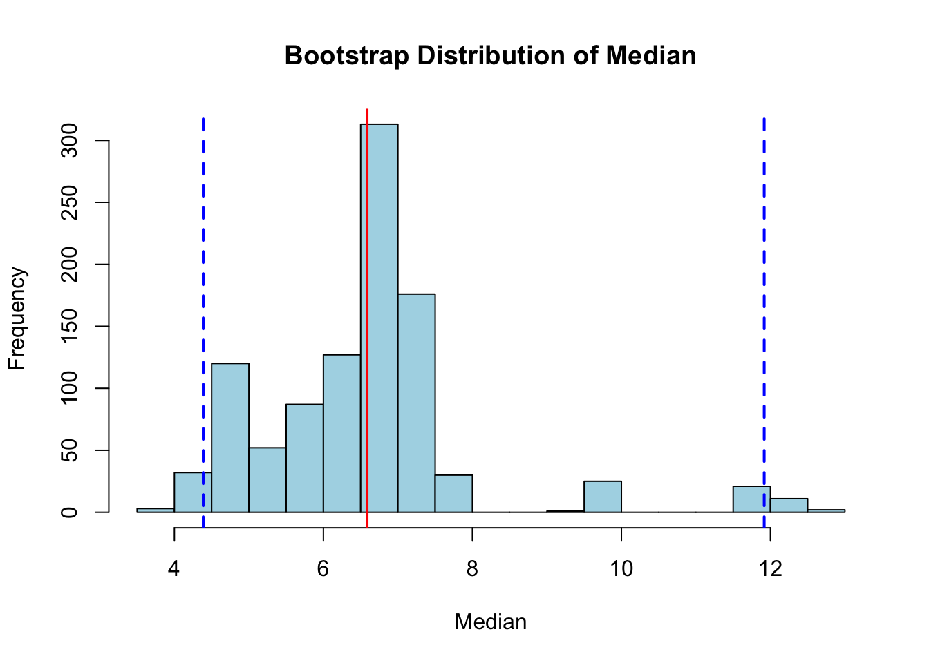
hist(boot_medians, breaks =30, main ="Bootstrap Distribution of Median",xlab ="Median", col ="lightblue")abline(v = observed_median, col ="red", lwd =2)abline(v = boot_ci, col ="blue", lwd =2, lty =2)
Figure 19.2: Bootstrap distribution of the median from 1000 resamples, showing the estimated sampling distribution with 95% confidence intervals
19.4 Advantages of the Bootstrap
The bootstrap is remarkably versatile. It can be applied to almost any statistic—means, medians, correlations, regression coefficients, eigenvalues, and more. It works when no formula for standard errors exists. It is nonparametric, making no assumptions about the underlying distribution. It handles complex sampling designs and calculations that would be intractable analytically.
The bootstrap is widely used for assessing confidence in phylogenetic trees, where the complexity of tree-building algorithms makes analytical approaches impractical. In machine learning, bootstrap aggregating (bagging) improves prediction accuracy by combining models trained on bootstrap samples.
19.5 When the Bootstrap Fails
The bootstrap is not a magic solution to all problems. It requires that the original sample be representative of the population—a biased sample produces biased bootstrap estimates. It can struggle with very small samples where the original data may not adequately represent the population.
Certain statistics, like the maximum of a sample, are poorly estimated by the bootstrap because the bootstrap distribution is bounded by the observed data. The bootstrap also assumes that observations are independent; for dependent data (like time series), specialized bootstrap methods are needed.
19.6 Bootstrap Confidence Intervals
Several methods exist for constructing bootstrap confidence intervals. The percentile method uses the quantiles of the bootstrap distribution directly. The basic bootstrap method reflects the bootstrap distribution around the observed estimate. The BCa (bias-corrected and accelerated) method adjusts for bias and skewness in the bootstrap distribution.
Code
# Different bootstrap CI methodslibrary(boot)# Define statistic functionmedian_fun <-function(data, indices) {median(data[indices])}# Run bootstrapboot_result <-boot(original_data, median_fun, R =1000)# Different CI methodsboot.ci(boot_result, type =c("perc", "basic", "bca"))
BOOTSTRAP CONFIDENCE INTERVAL CALCULATIONS
Based on 1000 bootstrap replicates

CALL :
boot.ci(boot.out = boot_result, type = c("perc", "basic", "bca"))

Intervals :
Level      Basic              Percentile            BCa
95%   ( 1.256,  8.841 )   ( 4.331, 11.916 )   ( 4.244, 11.582 )
Calculations and Intervals on Original Scale
The BCa method is generally preferred when computationally feasible, as it provides better coverage in many situations.
19.7 Practical Recommendations
For most applications, 1000 bootstrap replications provide adequate precision for standard errors. For confidence intervals, especially when using the BCa method, 10,000 replications may be preferable. Always set a random seed for reproducibility.
Remember that the bootstrap estimates sampling variability—it cannot fix problems with biased samples or invalid measurements. Use it as a tool for understanding uncertainty, not as a cure for poor data quality.
19.8 Permutation Tests
While the bootstrap estimates sampling variability by resampling with replacement, permutation tests (also called randomization tests) address a different question: they test the null hypothesis by resampling without replacement. Permutation tests are among the oldest statistical tests, predating many parametric methods.
The Permutation Idea
A permutation test asks: “If there were truly no difference between groups, how likely would we be to see a difference as large as the one we observed?”
Under the null hypothesis of no group difference, group labels are arbitrary—the data could have been assigned to either group. A permutation test generates the null distribution by repeatedly shuffling group labels and recalculating the test statistic. The p-value is the proportion of permuted statistics as extreme as the observed statistic.
Code
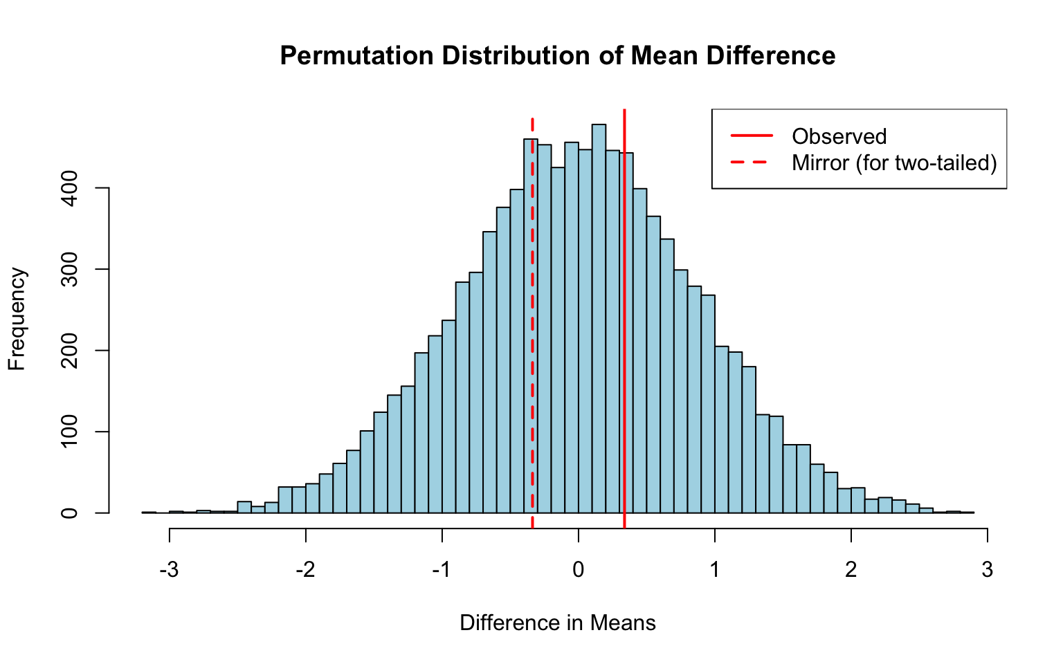
# Example: Two-sample permutation testset.seed(42)# Generate two groups with different meansgroup_A <-rnorm(15, mean =10, sd =2)group_B <-rnorm(15, mean =12, sd =2)# Observed difference in meansobserved_diff <-mean(group_B) -mean(group_A)cat("Observed difference:", round(observed_diff, 3), "\n")
Observed difference: 0.337
Code
# Combined data for permutationcombined <-c(group_A, group_B)n_A <-length(group_A)n_B <-length(group_B)n_total <- n_A + n_B# Permutation testn_perm <-10000perm_diffs <-replicate(n_perm, { shuffled <-sample(combined) # Shuffle without replacementmean(shuffled[(n_A +1):n_total]) -mean(shuffled[1:n_A])})# Visualize the permutation distributionhist(perm_diffs, breaks =50, col ="lightblue",main ="Permutation Distribution of Mean Difference",xlab ="Difference in Means")abline(v = observed_diff, col ="red", lwd =2)abline(v =-observed_diff, col ="red", lwd =2, lty =2)legend("topright", c("Observed", "Mirror (for two-tailed)"),col ="red", lty =c(1, 2), lwd =2)
Figure 19.3: Permutation test concept: if group labels don’t matter, shuffling them should produce similar results
Calculating the P-Value
Code
# Two-tailed p-value: proportion of permuted differences as extreme as observedp_value <-mean(abs(perm_diffs) >=abs(observed_diff))cat("Permutation p-value:", p_value, "\n")
Permutation p-value: 0.6947
Code
# Compare to t-testt_test <-t.test(group_B, group_A)cat("t-test p-value:", round(t_test$p.value, 4), "\n")
t-test p-value: 0.704
The permutation p-value and parametric p-value are often similar when parametric assumptions are met. The permutation test is exact—it gives the correct p-value regardless of the underlying distribution.
Permutation Test for Correlation
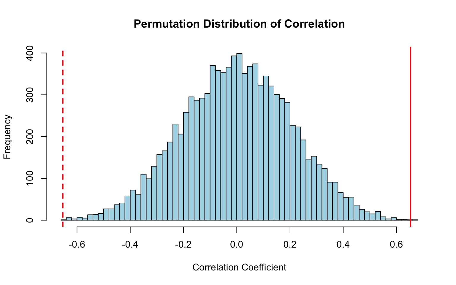
Permutation tests work for any test statistic. Here’s an example testing whether a correlation is significantly different from zero:
# Permutation test: shuffle one variable to break associationn_perm <-10000perm_cors <-replicate(n_perm, {cor(x, sample(y)) # Shuffle y, keeping x fixed})# Permutation p-valuep_value_cor <-mean(abs(perm_cors) >=abs(observed_cor))cat("Permutation p-value:", p_value_cor, "\n")
Permutation p-value: 1e-04
Code
# Visualizehist(perm_cors, breaks =50, col ="lightblue",main ="Permutation Distribution of Correlation",xlab ="Correlation Coefficient")abline(v = observed_cor, col ="red", lwd =2)abline(v =-observed_cor, col ="red", lwd =2, lty =2)
Figure 19.4: Permutation test for correlation: null distribution generated by breaking the X-Y pairing
Bootstrap vs Permutation
The bootstrap and permutation tests answer different questions:
Feature
Bootstrap
Permutation Test
Question
What is the sampling variability of my estimate?
Is the observed effect real or due to chance?
Resampling
With replacement
Without replacement
Output
Confidence intervals, standard errors
P-value
Null hypothesis
None assumed
Tests specific null (e.g., no group difference)
Assumptions
Sample is representative
Observations are exchangeable under null
Use bootstrap when: - You want confidence intervals for any statistic - No convenient formula for standard error exists - You need to assess uncertainty
Use permutation tests when: - You want to test a null hypothesis - Parametric assumptions may be violated - You want an exact test without distributional assumptions
Permutation Test for Paired Data
For paired designs (like before/after measurements), permute the sign of differences rather than shuffling between groups:
Code
# Paired permutation testset.seed(456)before <-rnorm(20, mean =100, sd =15)after <- before +rnorm(20, mean =5, sd =8) # Treatment adds ~5 units# Observed mean differencedifferences <- after - beforeobserved_mean_diff <-mean(differences)cat("Observed mean difference:", round(observed_mean_diff, 3), "\n")
Sample sizes are small: Parametric tests may not be reliable
Distributions are non-normal: Especially with skewed or heavy-tailed data
Data are ranks or ordinal: No parametric distribution applies
Complex test statistics: Custom statistics without known distributions
You want exact inference: No approximation error from asymptotic theory
Practical Considerations
Number of permutations: 10,000 is often sufficient; for publishable results, 100,000 gives more precision
Computation: Permutation tests can be slow for large datasets; consider parallel computing
Small samples: With very small samples, the number of unique permutations is limited
Exact vs. Monte Carlo: For small samples, you can enumerate all permutations exactly; for larger samples, random sampling (Monte Carlo) approximates the permutation distribution
Implementation with coin Package
The coin package provides efficient, well-tested permutation tests:
Code
library(coin)# Two-sample permutation testtest_data <-data.frame(value =c(group_A, group_B),group =factor(rep(c("A", "B"), c(length(group_A), length(group_B)))))# Exact permutation test (or Monte Carlo approximation for larger samples)oneway_test(value ~ group, data = test_data, distribution ="approximate")
    Approximative Two-Sample Fisher-Pitman Permutation Test

data:  value by group (A, B)
Z = -0.38996, p-value = 0.6972
alternative hypothesis: true mu is not equal to 0
19.9 Summary
Resampling methods provide powerful, flexible tools for statistical inference:
Bootstrap estimates sampling variability by resampling with replacement from observed data
Permutation tests test null hypotheses by resampling without replacement to generate null distributions
Both methods make minimal distributional assumptions
Bootstrap excels at constructing confidence intervals; permutation tests excel at hypothesis testing
Use 1,000+ replications for bootstrap standard errors; 10,000+ for confidence intervals and p-values
These methods complement rather than replace traditional parametric approaches
19.10 Exercises
Exercise B.1: Bootstrap Standard Errors
You measure the half-life of a radioactive isotope in 15 independent experiments:
Use the bootstrap (sampling with replacement from each group separately) to construct 95% CIs for the mean of group1 and the mean of group2
Use a permutation test to test whether the two groups have different means
Explain in your own words:
What question does the bootstrap answer?
What question does the permutation test answer?
Why do we resample WITH replacement for bootstrap but WITHOUT replacement for permutation tests?
Create visualizations demonstrating both the bootstrap distribution (for one of the means) and the permutation distribution (for the difference in means)
Code
# Your code here
Efron, Bradley. 1979. “Bootstrap Methods: Another Look at the Jackknife.”The Annals of Statistics 7 (1): 1–26.
Source Code
# Resampling Methods {#sec-bootstrapping}```{r}#| echo: false#| message: falselibrary(tidyverse)theme_set(theme_minimal())```## The Bootstrap IdeaFor the sample mean, we have elegant formulas for standard errors and confidence intervals derived from probability theory. But what about other statistics—the median, a correlation coefficient, the ratio of two means? For many estimators, no convenient formula exists.The bootstrap [@efron1979bootstrap], invented by Bradley Efron in 1979, provides a general solution. The key insight is that we can learn about the sampling distribution of a statistic by resampling from our data. If our sample is representative of the population, then samples drawn from our sample (with replacement) mimic what we would get from repeated sampling from the population.{#fig-bootstrap-resampling fig-align="center"}## Why the Bootstrap WorksThe bootstrap treats the observed sample as if it were the population. By drawing many samples with replacement from this "population," we create a distribution of the statistic of interest. This bootstrap distribution approximates the true sampling distribution.The bootstrap standard error is the standard deviation of the bootstrap distribution. Bootstrap confidence intervals can be constructed from the percentiles of the bootstrap distribution—the 2.5th and 97.5th percentiles give an approximate 95% confidence interval.## Bootstrap ProcedureThe basic algorithm is straightforward:1. Draw a random sample of size n from your data with replacement (the bootstrap sample)2. Calculate the statistic of interest from this bootstrap sample3. Repeat steps 1 and 2 many times (1000 or more)4. Use the distribution of bootstrap statistics to estimate standard error or confidence intervals```{r}#| label: fig-bootstrap-dist#| fig-cap: "Bootstrap distribution of the median from 1000 resamples, showing the estimated sampling distribution with 95% confidence intervals"#| fig-width: 7#| fig-height: 5# Bootstrap example: estimating standard error of medianset.seed(42)original_data <-rexp(50, rate =0.1) # Skewed distribution# Observed medianobserved_median <-median(original_data)# Bootstrapn_boot <-1000boot_medians <-replicate(n_boot, { boot_sample <-sample(original_data, replace =TRUE)median(boot_sample)})# Bootstrap standard errorboot_se <-sd(boot_medians)# Bootstrap confidence interval (percentile method)boot_ci <-quantile(boot_medians, c(0.025, 0.975))cat("Observed median:", round(observed_median, 2), "\n")cat("Bootstrap SE:", round(boot_se, 2), "\n")cat("95% CI:", round(boot_ci, 2), "\n")hist(boot_medians, breaks =30, main ="Bootstrap Distribution of Median",xlab ="Median", col ="lightblue")abline(v = observed_median, col ="red", lwd =2)abline(v = boot_ci, col ="blue", lwd =2, lty =2)```## Advantages of the BootstrapThe bootstrap is remarkably versatile. It can be applied to almost any statistic—means, medians, correlations, regression coefficients, eigenvalues, and more. It works when no formula for standard errors exists. It is nonparametric, making no assumptions about the underlying distribution. It handles complex sampling designs and calculations that would be intractable analytically.The bootstrap is widely used for assessing confidence in phylogenetic trees, where the complexity of tree-building algorithms makes analytical approaches impractical. In machine learning, bootstrap aggregating (bagging) improves prediction accuracy by combining models trained on bootstrap samples.## When the Bootstrap FailsThe bootstrap is not a magic solution to all problems. It requires that the original sample be representative of the population—a biased sample produces biased bootstrap estimates. It can struggle with very small samples where the original data may not adequately represent the population.Certain statistics, like the maximum of a sample, are poorly estimated by the bootstrap because the bootstrap distribution is bounded by the observed data. The bootstrap also assumes that observations are independent; for dependent data (like time series), specialized bootstrap methods are needed.## Bootstrap Confidence IntervalsSeveral methods exist for constructing bootstrap confidence intervals. The **percentile method** uses the quantiles of the bootstrap distribution directly. The **basic bootstrap** method reflects the bootstrap distribution around the observed estimate. The **BCa (bias-corrected and accelerated)** method adjusts for bias and skewness in the bootstrap distribution.```{r}# Different bootstrap CI methodslibrary(boot)# Define statistic functionmedian_fun <-function(data, indices) {median(data[indices])}# Run bootstrapboot_result <-boot(original_data, median_fun, R =1000)# Different CI methodsboot.ci(boot_result, type =c("perc", "basic", "bca"))```The BCa method is generally preferred when computationally feasible, as it provides better coverage in many situations.## Practical RecommendationsFor most applications, 1000 bootstrap replications provide adequate precision for standard errors. For confidence intervals, especially when using the BCa method, 10,000 replications may be preferable. Always set a random seed for reproducibility.Remember that the bootstrap estimates sampling variability—it cannot fix problems with biased samples or invalid measurements. Use it as a tool for understanding uncertainty, not as a cure for poor data quality.## Permutation TestsWhile the bootstrap estimates sampling variability by resampling **with replacement**, **permutation tests** (also called **randomization tests**) address a different question: they test the null hypothesis by resampling **without replacement**. Permutation tests are among the oldest statistical tests, predating many parametric methods.### The Permutation IdeaA permutation test asks: "If there were truly no difference between groups, how likely would we be to see a difference as large as the one we observed?"Under the null hypothesis of no group difference, group labels are arbitrary—the data could have been assigned to either group. A permutation test generates the null distribution by repeatedly shuffling group labels and recalculating the test statistic. The p-value is the proportion of permuted statistics as extreme as the observed statistic.```{r}#| label: fig-permutation-concept#| fig-cap: "Permutation test concept: if group labels don't matter, shuffling them should produce similar results"#| fig-width: 8#| fig-height: 5# Example: Two-sample permutation testset.seed(42)# Generate two groups with different meansgroup_A <-rnorm(15, mean =10, sd =2)group_B <-rnorm(15, mean =12, sd =2)# Observed difference in meansobserved_diff <-mean(group_B) -mean(group_A)cat("Observed difference:", round(observed_diff, 3), "\n")# Combined data for permutationcombined <-c(group_A, group_B)n_A <-length(group_A)n_B <-length(group_B)n_total <- n_A + n_B# Permutation testn_perm <-10000perm_diffs <-replicate(n_perm, { shuffled <-sample(combined) # Shuffle without replacementmean(shuffled[(n_A +1):n_total]) -mean(shuffled[1:n_A])})# Visualize the permutation distributionhist(perm_diffs, breaks =50, col ="lightblue",main ="Permutation Distribution of Mean Difference",xlab ="Difference in Means")abline(v = observed_diff, col ="red", lwd =2)abline(v =-observed_diff, col ="red", lwd =2, lty =2)legend("topright", c("Observed", "Mirror (for two-tailed)"),col ="red", lty =c(1, 2), lwd =2)```### Calculating the P-Value```{r}# Two-tailed p-value: proportion of permuted differences as extreme as observedp_value <-mean(abs(perm_diffs) >=abs(observed_diff))cat("Permutation p-value:", p_value, "\n")# Compare to t-testt_test <-t.test(group_B, group_A)cat("t-test p-value:", round(t_test$p.value, 4), "\n")```The permutation p-value and parametric p-value are often similar when parametric assumptions are met. The permutation test is exact—it gives the correct p-value regardless of the underlying distribution.### Permutation Test for CorrelationPermutation tests work for any test statistic. Here's an example testing whether a correlation is significantly different from zero:```{r}#| label: fig-permutation-correlation#| fig-cap: "Permutation test for correlation: null distribution generated by breaking the X-Y pairing"#| fig-width: 8#| fig-height: 5# Test correlation significanceset.seed(123)x <-rnorm(25)y <-0.5* x +rnorm(25, sd =0.8) # True correlation exists# Observed correlationobserved_cor <-cor(x, y)cat("Observed correlation:", round(observed_cor, 3), "\n")# Permutation test: shuffle one variable to break associationn_perm <-10000perm_cors <-replicate(n_perm, {cor(x, sample(y)) # Shuffle y, keeping x fixed})# Permutation p-valuep_value_cor <-mean(abs(perm_cors) >=abs(observed_cor))cat("Permutation p-value:", p_value_cor, "\n")# Visualizehist(perm_cors, breaks =50, col ="lightblue",main ="Permutation Distribution of Correlation",xlab ="Correlation Coefficient")abline(v = observed_cor, col ="red", lwd =2)abline(v =-observed_cor, col ="red", lwd =2, lty =2)```### Bootstrap vs PermutationThe bootstrap and permutation tests answer different questions:| Feature | Bootstrap | Permutation Test ||:--------|:----------|:-----------------|| **Question** | What is the sampling variability of my estimate? | Is the observed effect real or due to chance? || **Resampling** | With replacement | Without replacement || **Output** | Confidence intervals, standard errors | P-value || **Null hypothesis** | None assumed | Tests specific null (e.g., no group difference) || **Assumptions** | Sample is representative | Observations are exchangeable under null |**Use bootstrap when:**- You want confidence intervals for any statistic- No convenient formula for standard error exists- You need to assess uncertainty**Use permutation tests when:**- You want to test a null hypothesis- Parametric assumptions may be violated- You want an exact test without distributional assumptions### Permutation Test for Paired DataFor paired designs (like before/after measurements), permute the sign of differences rather than shuffling between groups:```{r}# Paired permutation testset.seed(456)before <-rnorm(20, mean =100, sd =15)after <- before +rnorm(20, mean =5, sd =8) # Treatment adds ~5 units# Observed mean differencedifferences <- after - beforeobserved_mean_diff <-mean(differences)cat("Observed mean difference:", round(observed_mean_diff, 3), "\n")# Permutation: randomly flip signs of differencesn_perm <-10000perm_means <-replicate(n_perm, { signs <-sample(c(-1, 1), length(differences), replace =TRUE)mean(differences * signs)})# P-valuep_value_paired <-mean(abs(perm_means) >=abs(observed_mean_diff))cat("Permutation p-value:", p_value_paired, "\n")# Compare to paired t-testpaired_t <-t.test(after, before, paired =TRUE)cat("Paired t-test p-value:", round(paired_t$p.value, 4), "\n")```### When Permutation Tests ExcelPermutation tests are particularly valuable when:1. **Sample sizes are small**: Parametric tests may not be reliable2. **Distributions are non-normal**: Especially with skewed or heavy-tailed data3. **Data are ranks or ordinal**: No parametric distribution applies4. **Complex test statistics**: Custom statistics without known distributions5. **You want exact inference**: No approximation error from asymptotic theory::: {.callout-tip}## Practical Considerations- **Number of permutations**: 10,000 is often sufficient; for publishable results, 100,000 gives more precision- **Computation**: Permutation tests can be slow for large datasets; consider parallel computing- **Small samples**: With very small samples, the number of unique permutations is limited- **Exact vs. Monte Carlo**: For small samples, you can enumerate all permutations exactly; for larger samples, random sampling (Monte Carlo) approximates the permutation distribution:::### Implementation with coin PackageThe `coin` package provides efficient, well-tested permutation tests:```{r}library(coin)# Two-sample permutation testtest_data <-data.frame(value =c(group_A, group_B),group =factor(rep(c("A", "B"), c(length(group_A), length(group_B)))))# Exact permutation test (or Monte Carlo approximation for larger samples)oneway_test(value ~ group, data = test_data, distribution ="approximate")```## SummaryResampling methods provide powerful, flexible tools for statistical inference:- **Bootstrap** estimates sampling variability by resampling with replacement from observed data- **Permutation tests** test null hypotheses by resampling without replacement to generate null distributions- Both methods make minimal distributional assumptions- Bootstrap excels at constructing confidence intervals; permutation tests excel at hypothesis testing- Use 1,000+ replications for bootstrap standard errors; 10,000+ for confidence intervals and p-values- These methods complement rather than replace traditional parametric approaches## Exercises::: {.callout-note}### Exercise B.1: Bootstrap Standard ErrorsYou measure the half-life of a radioactive isotope in 15 independent experiments:```half_lives <- c(5.2, 5.8, 5.1, 6.2, 5.9, 5.4, 6.1, 5.7, 5.3, 6.0, 5.5, 5.9, 5.6, 6.3, 5.4)```a) Calculate the mean and median half-lifeb) Use the bootstrap (with 5000 replications) to estimate the standard error of the meanc) Use the bootstrap to estimate the standard error of the mediand) Compare the bootstrap SE of the mean to the analytical formula SE = s/√ne) Create histograms of the bootstrap distributions for both the mean and medianf) Which statistic (mean or median) has greater sampling variability for these data?```{r}#| eval: false# Your code here```:::::: {.callout-note}### Exercise B.2: Bootstrap Confidence IntervalsYou measure reaction times (in milliseconds) for a cognitive task:```reaction_times <- c(234, 245, 267, 289, 256, 298, 312, 245, 278, 301, 267, 289, 234, 256, 278)```a) Calculate 95% confidence intervals for the median using three methods: - Percentile method (manual calculation) - Using the `boot` package with percentile, basic, and BCa methodsb) Compare the widths and endpoints of these different confidence intervalsc) Which method would you prefer for this dataset and why?d) Bootstrap the 90th percentile and construct a 95% CI for it```{r}#| eval: false# Your code herelibrary(boot)```:::::: {.callout-note}### Exercise B.3: Bootstrap for CorrelationYou have measurements of two physiological variables:```x <- c(12.3, 14.5, 11.8, 15.2, 13.1, 14.8, 12.9, 15.5, 13.6, 14.1)y <- c(98, 105, 95, 110, 101, 107, 99, 112, 103, 106)```a) Calculate Pearson's correlation coefficientb) Calculate the 95% CI for the correlation using the traditional Fisher z-transformation method (`cor.test()`)c) Use the bootstrap (10000 replications) to construct a 95% CI for the correlationd) Compare the two confidence intervals—are they similar?e) Create a scatterplot with the data and report the correlation with its bootstrap CI```{r}#| eval: false# Your code here```:::::: {.callout-note}### Exercise B.4: Permutation Test vs. t-testYou compare growth rates of bacteria cultured in two different media:```medium_A <- c(0.42, 0.38, 0.45, 0.41, 0.39, 0.44, 0.40, 0.43)medium_B <- c(0.51, 0.48, 0.55, 0.49, 0.52, 0.47, 0.54, 0.50)```a) Visualize the two groups with boxplotsb) Perform a two-sample t-testc) Implement a permutation test with 10,000 permutations to test for a difference in meansd) Compare the p-values from the t-test and permutation teste) Calculate the effect size (Cohen's d)f) Createhistogram of the permutation distribution with the observed difference marked```{r}#| eval: false# Your code here```:::::: {.callout-note}### Exercise B.5: Paired Permutation TestYou measure expression levels of a gene before and after heat stress in 10 plant samples:```before_stress <- c(125, 142, 138, 151, 129, 145, 133, 148, 136, 141)after_stress <- c(189, 207, 195, 218, 182, 203, 191, 214, 198, 206)```a) Calculate the paired differences and perform a paired t-testb) Implement a paired permutation test by randomly flipping the signs of differences (10,000 permutations)c) Compare the p-values from both methodsd) Use the bootstrap to construct a 95% CI for the mean differencee) Visualize the paired data with a before-after plot (connecting lines between paired points)```{r}#| eval: false# Your code here```:::::: {.callout-note}### Exercise B.6: Bootstrap vs. Permutation—Understanding the DifferenceConsider the following dataset:```group1 <- c(23, 25, 28, 31, 27, 29, 26, 30)group2 <- c(35, 38, 33, 40, 36, 37, 34, 39)```a) Use the bootstrap (sampling with replacement from each group separately) to construct 95% CIs for the mean of group1 and the mean of group2b) Use a permutation test to test whether the two groups have different meansc) Explain in your own words: - What question does the bootstrap answer? - What question does the permutation test answer? - Why do we resample WITH replacement for bootstrap but WITHOUT replacement for permutation tests?d) Create visualizations demonstrating both the bootstrap distribution (for one of the means) and the permutation distribution (for the difference in means)```{r}#| eval: false# Your code here```:::