27 Single Factor ANOVA

27.1 Beyond Two Groups

The t-test compares two groups, but many experiments involve more than two. We might compare three drug treatments, five temperature conditions, or four genetic strains. Running multiple t-tests creates problems: with many comparisons, false positives become likely even when no true differences exist.

Analysis of Variance (ANOVA) provides a solution. It tests whether any of the group means differ from the others in a single test, controlling the overall Type I error rate.

27.2 The ANOVA Framework

Analysis of Variance (ANOVA), developed by Ronald A. Fisher (Fisher 1925), partitions the total variation in the data into components: variation between groups (due to treatment effects) and variation within groups (due to random error).

Figure 27.1: ANOVA partitions total variation into between-group and within-group components

The key insight is that if groups have equal means, the between-group variation should be similar to the within-group variation. If the between-group variation is much larger, the group means probably differ.

Figure 27.2: Comparison of between-group and within-group variation under different scenarios

27.3 The F-Test

ANOVA uses the F-statistic:

\[F = \frac{MS_{between}}{MS_{within}} = \frac{\text{Variance between groups}}{\text{Variance within groups}}\]

Under the null hypothesis (all group means equal), F follows an F-distribution. Large F values indicate that group means differ more than expected by chance.

27.4 One-Way ANOVA in R

Code

# Example using iris data
iris_aov <- aov(Sepal.Length ~ Species, data = iris)
summary(iris_aov)

             Df Sum Sq Mean Sq F value Pr(>F)    
Species       2  63.21  31.606   119.3 <2e-16 ***
Residuals   147  38.96   0.265                   
---
Signif. codes:  0 '***' 0.001 '**' 0.01 '*' 0.05 '.' 0.1 ' ' 1

The significant p-value tells us that sepal length differs among species, but not which species differ from which.

27.5 ANOVA Assumptions

Like the t-test, ANOVA assumes:

Normality: Observations within each group are normally distributed
Homogeneity of variance: Groups have equal variances
Independence: Observations are independent

ANOVA is robust to mild violations of normality, especially with balanced designs and large samples. Serious violations of homogeneity of variance are more problematic but can be addressed with Welch’s ANOVA or transformations.

27.6 Post-Hoc Comparisons

A significant ANOVA tells us groups differ but not how. Post-hoc tests compare specific pairs of groups while controlling for multiple comparisons.

Tukey’s HSD (Honestly Significant Difference) compares all pairs:

Code

TukeyHSD(iris_aov)

  Tukey multiple comparisons of means
    95% family-wise confidence level

Fit: aov(formula = Sepal.Length ~ Species, data = iris)

$Species
                      diff       lwr       upr p adj
versicolor-setosa    0.930 0.6862273 1.1737727     0
virginica-setosa     1.582 1.3382273 1.8257727     0
virginica-versicolor 0.652 0.4082273 0.8957727     0

Each pairwise comparison includes the difference in means, confidence interval, and adjusted p-value.

27.7 Planned Contrasts

If you have specific hypotheses about which groups should differ (decided before seeing the data), planned contrasts are more powerful than post-hoc tests. They focus statistical power on the comparisons you care about.

Code

# Example: Compare setosa to the average of the other two species
contrasts(iris$Species) <- cbind(
  setosa_vs_others = c(2, -1, -1)
)
summary.lm(aov(Sepal.Length ~ Species, data = iris))


Call:
aov(formula = Sepal.Length ~ Species, data = iris)

Residuals:
    Min      1Q  Median      3Q     Max 
-1.6880 -0.3285 -0.0060  0.3120  1.3120 

Coefficients:
                        Estimate Std. Error t value Pr(>|t|)    
(Intercept)              5.84333    0.04203 139.020  < 2e-16 ***
Speciessetosa_vs_others -0.41867    0.02972 -14.086  < 2e-16 ***
Species                  0.46103    0.07280   6.333 2.77e-09 ***
---
Signif. codes:  0 '***' 0.001 '**' 0.01 '*' 0.05 '.' 0.1 ' ' 1

Residual standard error: 0.5148 on 147 degrees of freedom
Multiple R-squared:  0.6187,    Adjusted R-squared:  0.6135 
F-statistic: 119.3 on 2 and 147 DF,  p-value: < 2.2e-16

27.8 Fixed vs. Random Effects

Fixed effects are specific treatments of interest that would be the same if the study were replicated—drug A, drug B, drug C. Conclusions apply only to these specific treatments.

Random effects are levels sampled from a larger population—particular subjects, batches, or locations. The goal is to generalize to the population of possible levels, not just those observed.

The distinction matters because it affects how F-ratios are calculated and what conclusions can be drawn.

27.9 Effect Sizes in ANOVA

Beyond statistical significance, report how much of the variance is explained by your factors.

Eta-squared ($\eta^2$): Proportion of total variance explained by the factor

\[\eta^2 = \frac{SS_{between}}{SS_{total}}\]

Partial eta-squared ($\eta^2_p$): Proportion of variance explained after accounting for other factors

Omega-squared ($\omega^2$): Less biased estimate of variance explained in the population

Code

# Calculate effect sizes
ss <- summary(iris_aov)[[1]]
ss_between <- ss["Species", "Sum Sq"]
ss_within <- ss["Residuals", "Sum Sq"]
ss_total <- ss_between + ss_within

eta_squared <- ss_between / ss_total
cat("Eta-squared:", round(eta_squared, 3), "\n")

Eta-squared: 0.619

Code

# Omega-squared (less biased)
ms_within <- ss["Residuals", "Mean Sq"]
n <- nrow(iris)
k <- length(unique(iris$Species))
omega_squared <- (ss_between - (k-1) * ms_within) / (ss_total + ms_within)
cat("Omega-squared:", round(omega_squared, 3), "\n")

Omega-squared: 0.612

27.10 Pseudoreplication

A Common Design Flaw

Pseudoreplication occurs when non-independent observations are treated as independent replicates. This inflates the apparent sample size and leads to artificially small p-values.

Common examples: - Multiple measurements from the same individual treated as independent - Multiple cells from the same culture dish - Multiple fish from the same tank when treatment was applied to tanks - Technical replicates confused with biological replicates

The unit of replication must be the unit to which the treatment was independently applied. If you treat three tanks with drug A and three with drug B, you have n=3 per group regardless of how many fish are in each tank.

Code

# Wrong: treats individual fish as independent
# If 10 fish per tank, and tanks are the true units:
set.seed(42)
# This overstates the evidence because fish within tanks are correlated
tank_A <- rep(c(10, 12, 11), each = 10) + rnorm(30, sd = 1)  # 3 tanks, 10 fish each
tank_B <- rep(c(8, 9, 8.5), each = 10) + rnorm(30, sd = 1)

# Pseudoreplicated analysis (WRONG - n appears to be 30 per group)
cat("Pseudoreplicated p-value:", t.test(tank_A, tank_B)$p.value, "\n")

Pseudoreplicated p-value: 2.315344e-11

Code

# Correct analysis (using tank means, n = 3 per group)
means_A <- c(mean(tank_A[1:10]), mean(tank_A[11:20]), mean(tank_A[21:30]))
means_B <- c(mean(tank_B[1:10]), mean(tank_B[11:20]), mean(tank_B[21:30]))
cat("Correct p-value:", t.test(means_A, means_B)$p.value, "\n")

Correct p-value: 0.008405113

The correct analysis has less power (larger p-value) because it honestly reflects the true sample size.

27.11 ANOVA as a General Linear Model

ANOVA is a special case of the general linear model (GLM). Both t-tests and ANOVA can be expressed as regression with indicator variables (dummy coding). This unified framework shows that these seemingly different methods are fundamentally the same.

Code

# ANOVA using lm() with dummy coding
# Equivalent to aov()
iris_lm <- lm(Sepal.Length ~ Species, data = iris)
anova(iris_lm)

Analysis of Variance Table

Response: Sepal.Length
           Df Sum Sq Mean Sq F value    Pr(>F)    
Species     2 63.212  31.606  119.26 < 2.2e-16 ***
Residuals 147 38.956   0.265                      
---
Signif. codes:  0 '***' 0.001 '**' 0.01 '*' 0.05 '.' 0.1 ' ' 1

The connection becomes clear when you realize: - A one-sample t-test is regression on an intercept - A two-sample t-test is regression with one binary predictor - One-way ANOVA is regression with multiple indicator variables

This unified view is powerful: once you understand regression, you understand the entire family of linear models.

27.12 Practice Exercises

Exercise 1: Plant Growth Analysis

The PlantGrowth dataset in R contains weights of plants obtained under three different conditions: control, treatment 1, and treatment 2.

Perform a one-way ANOVA to test whether the treatments affect plant weight
Check the assumptions using appropriate diagnostic plots
If the ANOVA is significant, perform Tukey’s HSD to identify which groups differ
Calculate and interpret the eta-squared effect size
Visualize the results with a boxplot or violin plot

Exercise 2: Diet and Weight Loss

A researcher tests four different diets on 40 participants (10 per diet). After 8 weeks, weight loss (in kg) is recorded. Create a simulated dataset and:

Perform a one-way ANOVA
Test the homogeneity of variance assumption using Levene’s test
Perform post-hoc comparisons using Tukey’s HSD
Calculate omega-squared to estimate the population effect size
Write a brief interpretation of the results

Exercise 3: Planned Contrasts

Using the chickwts dataset, which contains chicken weights for different feed supplements:

Examine the feed types and formulate two specific contrasts before analysis
Perform a one-way ANOVA
Test your planned contrasts
Compare the p-values from planned contrasts to post-hoc tests
Discuss why planned contrasts might be preferable when you have specific hypotheses

Exercise 4: Pseudoreplication Detection

A student measures enzyme activity in cells. They have 3 culture dishes per treatment (control and experimental), with 20 cells measured per dish.

What is the true sample size for each treatment?
What would happen to the p-value if cells were incorrectly treated as independent replicates?
Write R code to demonstrate the difference between the pseudoreplicated and correct analysis
Explain how you would properly analyze this experiment

Exercise 5: ANOVA as Regression

Using the iris dataset:

Perform a one-way ANOVA using aov() to test for differences in Petal.Length across species
Perform the same analysis using lm() and compare the results
Examine the coefficients from the lm() model and interpret what they represent
Use anova() on the lm() object to get the ANOVA table
Explain how the regression framework relates to the ANOVA framework

27.13 Summary

Single-factor ANOVA provides a framework for comparing means across multiple groups:

One-way ANOVA tests whether any group means differ in a single test
The F-test assesses whether between-group variance exceeds within-group variance
Post-hoc tests identify which specific groups differ while controlling for multiple comparisons
Planned contrasts are more powerful when you have specific hypotheses
Fixed effects are specific treatments; random effects are sampled from populations
Effect sizes (eta-squared, omega-squared) quantify the proportion of variance explained
Pseudoreplication is a critical design flaw that must be avoided
ANOVA is a special case of the general linear model

Always check assumptions, report effect sizes alongside p-values, and ensure your unit of analysis matches your unit of replication.

# Single Factor ANOVA {#sec-single-factor-anova} ```{r} #| echo: false #| message: false library(tidyverse) theme_set(theme_minimal()) ``` ## Beyond Two Groups The t-test compares two groups, but many experiments involve more than two. We might compare three drug treatments, five temperature conditions, or four genetic strains. Running multiple t-tests creates problems: with many comparisons, false positives become likely even when no true differences exist. Analysis of Variance (ANOVA) provides a solution. It tests whether any of the group means differ from the others in a single test, controlling the overall Type I error rate. ## The ANOVA Framework Analysis of Variance (ANOVA), developed by Ronald A. Fisher [@fisher1925statistical], partitions the total variation in the data into components: variation between groups (due to treatment effects) and variation within groups (due to random error).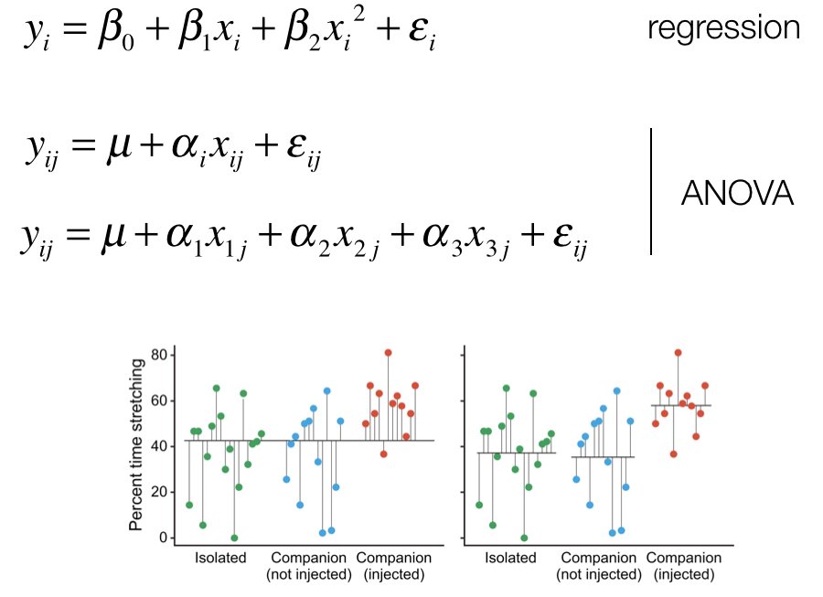 ![ANOVA partitions total variation into between-group and within-group components](../images/ch25/ch25_anova_partition.jpeg){#fig-anova-partition fig-align="center"} The key insight is that if groups have equal means, the between-group variation should be similar to the within-group variation. If the between-group variation is much larger, the group means probably differ.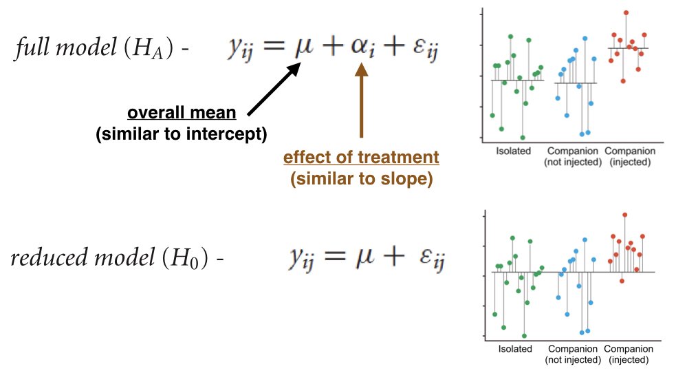 ![Comparison of between-group and within-group variation under different scenarios](../images/ch25/ch25_anova_variation.jpeg){#fig-anova-variation fig-align="center"} ## The F-Test ANOVA uses the F-statistic: $$F = \frac{MS_{between}}{MS_{within}} = \frac{\text{Variance between groups}}{\text{Variance within groups}}$$ Under the null hypothesis (all group means equal), F follows an F-distribution. Large F values indicate that group means differ more than expected by chance. ## One-Way ANOVA in R ```{r} # Example using iris data iris_aov <- aov(Sepal.Length ~ Species, data = iris) summary(iris_aov) ``` The significant p-value tells us that sepal length differs among species, but not which species differ from which. ## ANOVA Assumptions Like the t-test, ANOVA assumes: 1. **Normality**: Observations within each group are normally distributed 2. **Homogeneity of variance**: Groups have equal variances 3. **Independence**: Observations are independent ANOVA is robust to mild violations of normality, especially with balanced designs and large samples. Serious violations of homogeneity of variance are more problematic but can be addressed with Welch's ANOVA or transformations. ## Post-Hoc Comparisons A significant ANOVA tells us groups differ but not how. **Post-hoc tests** compare specific pairs of groups while controlling for multiple comparisons. **Tukey's HSD** (Honestly Significant Difference) compares all pairs: ```{r} TukeyHSD(iris_aov) ``` Each pairwise comparison includes the difference in means, confidence interval, and adjusted p-value. ## Planned Contrasts If you have specific hypotheses about which groups should differ (decided before seeing the data), planned contrasts are more powerful than post-hoc tests. They focus statistical power on the comparisons you care about. ```{r} # Example: Compare setosa to the average of the other two species contrasts(iris$Species) <- cbind( setosa_vs_others = c(2, -1, -1) ) summary.lm(aov(Sepal.Length ~ Species, data = iris)) ``` ## Fixed vs. Random Effects **Fixed effects** are specific treatments of interest that would be the same if the study were replicated—drug A, drug B, drug C. Conclusions apply only to these specific treatments. **Random effects** are levels sampled from a larger population—particular subjects, batches, or locations. The goal is to generalize to the population of possible levels, not just those observed. The distinction matters because it affects how F-ratios are calculated and what conclusions can be drawn. ## Effect Sizes in ANOVA Beyond statistical significance, report how much of the variance is explained by your factors. **Eta-squared ($\eta^2$)**: Proportion of total variance explained by the factor $$\eta^2 = \frac{SS_{between}}{SS_{total}}$$ **Partial eta-squared ($\eta^2_p$)**: Proportion of variance explained after accounting for other factors **Omega-squared ($\omega^2$)**: Less biased estimate of variance explained in the population ```{r} # Calculate effect sizes ss <- summary(iris_aov)[[1]] ss_between <- ss["Species", "Sum Sq"] ss_within <- ss["Residuals", "Sum Sq"] ss_total <- ss_between + ss_within eta_squared <- ss_between / ss_total cat("Eta-squared:", round(eta_squared, 3), "\n") # Omega-squared (less biased) ms_within <- ss["Residuals", "Mean Sq"] n <- nrow(iris) k <- length(unique(iris$Species)) omega_squared <- (ss_between - (k-1) * ms_within) / (ss_total + ms_within) cat("Omega-squared:", round(omega_squared, 3), "\n") ``` ## Pseudoreplication ::: {.callout-warning} ## A Common Design Flaw **Pseudoreplication** occurs when non-independent observations are treated as independent replicates. This inflates the apparent sample size and leads to artificially small p-values. Common examples: - Multiple measurements from the same individual treated as independent - Multiple cells from the same culture dish - Multiple fish from the same tank when treatment was applied to tanks - Technical replicates confused with biological replicates ::: The unit of replication must be the unit to which the treatment was independently applied. If you treat three tanks with drug A and three with drug B, you have n=3 per group regardless of how many fish are in each tank. ```{r} # Wrong: treats individual fish as independent # If 10 fish per tank, and tanks are the true units: set.seed(42) # This overstates the evidence because fish within tanks are correlated tank_A <- rep(c(10, 12, 11), each = 10) + rnorm(30, sd = 1) # 3 tanks, 10 fish each tank_B <- rep(c(8, 9, 8.5), each = 10) + rnorm(30, sd = 1) # Pseudoreplicated analysis (WRONG - n appears to be 30 per group) cat("Pseudoreplicated p-value:", t.test(tank_A, tank_B)$p.value, "\n") # Correct analysis (using tank means, n = 3 per group) means_A <- c(mean(tank_A[1:10]), mean(tank_A[11:20]), mean(tank_A[21:30])) means_B <- c(mean(tank_B[1:10]), mean(tank_B[11:20]), mean(tank_B[21:30])) cat("Correct p-value:", t.test(means_A, means_B)$p.value, "\n") ``` The correct analysis has less power (larger p-value) because it honestly reflects the true sample size. ## ANOVA as a General Linear Model ANOVA is a special case of the general linear model (GLM). Both t-tests and ANOVA can be expressed as regression with indicator variables (dummy coding). This unified framework shows that these seemingly different methods are fundamentally the same. ```{r} # ANOVA using lm() with dummy coding # Equivalent to aov() iris_lm <- lm(Sepal.Length ~ Species, data = iris) anova(iris_lm) ``` The connection becomes clear when you realize: - A one-sample t-test is regression on an intercept - A two-sample t-test is regression with one binary predictor - One-way ANOVA is regression with multiple indicator variables This unified view is powerful: once you understand regression, you understand the entire family of linear models. ## Practice Exercises ::: {.callout-note icon=false} ## Exercise 1: Plant Growth Analysis The `PlantGrowth` dataset in R contains weights of plants obtained under three different conditions: control, treatment 1, and treatment 2. a. Perform a one-way ANOVA to test whether the treatments affect plant weight b. Check the assumptions using appropriate diagnostic plots c. If the ANOVA is significant, perform Tukey's HSD to identify which groups differ d. Calculate and interpret the eta-squared effect size e. Visualize the results with a boxplot or violin plot ::: ::: {.callout-note icon=false} ## Exercise 2: Diet and Weight Loss A researcher tests four different diets on 40 participants (10 per diet). After 8 weeks, weight loss (in kg) is recorded. Create a simulated dataset and: a. Perform a one-way ANOVA b. Test the homogeneity of variance assumption using Levene's test c. Perform post-hoc comparisons using Tukey's HSD d. Calculate omega-squared to estimate the population effect size e. Write a brief interpretation of the results ::: ::: {.callout-note icon=false} ## Exercise 3: Planned Contrasts Using the `chickwts` dataset, which contains chicken weights for different feed supplements: a. Examine the feed types and formulate two specific contrasts before analysis b. Perform a one-way ANOVA c. Test your planned contrasts d. Compare the p-values from planned contrasts to post-hoc tests e. Discuss why planned contrasts might be preferable when you have specific hypotheses ::: ::: {.callout-note icon=false} ## Exercise 4: Pseudoreplication Detection A student measures enzyme activity in cells. They have 3 culture dishes per treatment (control and experimental), with 20 cells measured per dish. a. What is the true sample size for each treatment? b. What would happen to the p-value if cells were incorrectly treated as independent replicates? c. Write R code to demonstrate the difference between the pseudoreplicated and correct analysis d. Explain how you would properly analyze this experiment ::: ::: {.callout-note icon=false} ## Exercise 5: ANOVA as Regression Using the `iris` dataset: a. Perform a one-way ANOVA using `aov()` to test for differences in `Petal.Length` across species b. Perform the same analysis using `lm()` and compare the results c. Examine the coefficients from the `lm()` model and interpret what they represent d. Use `anova()` on the `lm()` object to get the ANOVA table e. Explain how the regression framework relates to the ANOVA framework ::: ## Summary Single-factor ANOVA provides a framework for comparing means across multiple groups: - One-way ANOVA tests whether any group means differ in a single test - The F-test assesses whether between-group variance exceeds within-group variance - Post-hoc tests identify which specific groups differ while controlling for multiple comparisons - Planned contrasts are more powerful when you have specific hypotheses - Fixed effects are specific treatments; random effects are sampled from populations - Effect sizes (eta-squared, omega-squared) quantify the proportion of variance explained - Pseudoreplication is a critical design flaw that must be avoided - ANOVA is a special case of the general linear model Always check assumptions, report effect sizes alongside p-values, and ensure your unit of analysis matches your unit of replication.