29 Generalized Linear Models

29.1 Beyond Normal Distributions

Standard linear regression assumes that the response variable is continuous and normally distributed. But many important response variables violate these assumptions. Binary outcomes (success/failure, alive/dead) follow binomial distributions. Count data (number of events, cells, species) often follow Poisson distributions.

Generalized Linear Models (GLMs) extend linear regression to handle these situations. They provide a unified framework for modeling responses that follow different distributions from the exponential family.

29.2 Frequency Analysis: Categorical Response Variables

Before diving into GLMs, it’s important to understand how we analyze categorical response variables. When observations fall into categories rather than being measured on a continuous scale, we count the frequency in each category and compare observed frequencies to expected values.

Chi-Square Goodness of Fit Test

The goodness of fit test asks whether observed frequencies match a hypothesized distribution. The classic example comes from Mendelian genetics.

Code

# Mendel's pea experiment - F2 phenotype ratios
# Expected: 9:3:3:1 for Yellow-Smooth:Yellow-Wrinkled:Green-Smooth:Green-Wrinkled
observed <- c(315, 101, 108, 32)  # Mendel's actual data
expected_ratios <- c(9/16, 3/16, 3/16, 1/16)

# Perform chi-square test
chisq.test(observed, p = expected_ratios)


    Chi-squared test for given probabilities

data:  observed
X-squared = 0.47002, df = 3, p-value = 0.9254

The test statistic measures deviation from expected:

\[\chi^2 = \sum \frac{(O_i - E_i)^2}{E_i}\]

where $O_i$ are observed and $E_i$ are expected counts. Under the null hypothesis (observed frequencies match expected), this follows a chi-square distribution with $df = k - 1$ where $k$ is the number of categories.

Chi-Square Assumptions

Independence: Observations must be independent
Expected counts: No more than 20% of expected counts should be < 5
Sample size: Total sample should be reasonably large

Check expected values before interpreting results:

Code

n <- sum(observed)
expected <- n * expected_ratios
cat("Expected counts:", round(expected, 1))

Expected counts: 312.8 104.2 104.2 34.8

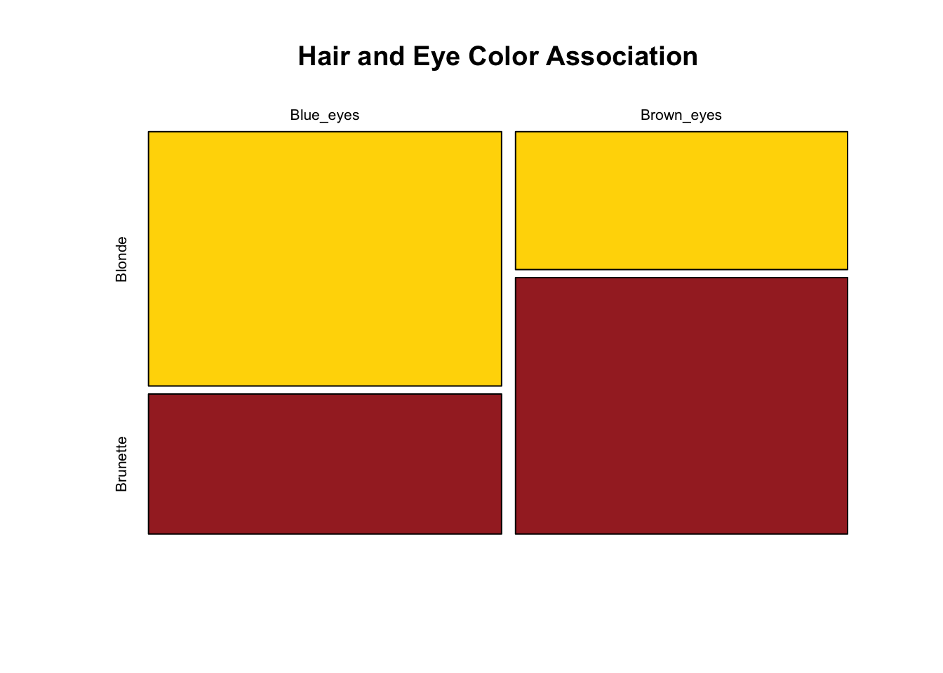
Contingency Table Analysis

When we have two categorical variables, we use a contingency table to examine their association. The null hypothesis is that the variables are independent.

Code

# Example: Hair color and eye color association
# Data from 1000 students
hair_eye <- matrix(c(347, 191,    # Blue eyes: blonde, brunette
                     177, 329),   # Brown eyes: blonde, brunette
                   nrow = 2, byrow = TRUE)
rownames(hair_eye) <- c("Blue_eyes", "Brown_eyes")
colnames(hair_eye) <- c("Blonde", "Brunette")

# View the contingency table
hair_eye

           Blonde Brunette
Blue_eyes     347      191
Brown_eyes    177      329

Code

# Chi-square test of independence
chisq.test(hair_eye)


    Pearson's Chi-squared test with Yates' continuity correction

data:  hair_eye
X-squared = 89.703, df = 1, p-value < 2.2e-16

For contingency tables, $df = (r-1)(c-1)$ where $r$ and $c$ are the number of rows and columns.

Code

# Visualize with a mosaic plot
mosaicplot(hair_eye, main = "Hair and Eye Color Association",
           color = c("gold", "brown"), shade = FALSE)

Figure 29.1: Mosaic plot showing the association between hair color and eye color

Standardized Residuals

To understand where associations are strongest, examine standardized residuals:

Code

# Which cells deviate most from independence?
test_result <- chisq.test(hair_eye)
test_result$residuals

              Blonde  Brunette
Blue_eyes   4.683940 -4.701920
Brown_eyes -4.829778  4.848318

Residuals > 2 or < -2 indicate cells contributing substantially to the association. Positive residuals mean more observations than expected under independence; negative means fewer.

G-Test (Log-Likelihood Ratio Test)

The G-test is an alternative to chi-square based on likelihood ratios:

\[G = 2 \sum O_i \ln\left(\frac{O_i}{E_i}\right)\]

The G-test and chi-square give similar results for large samples, but G-tests are preferred when: - Sample sizes are small - Differences between observed and expected are small - You want to decompose complex tables

Code

# Manual G-test calculation
observed_flat <- as.vector(hair_eye)
expected_flat <- as.vector(test_result$expected)
G <- 2 * sum(observed_flat * log(observed_flat / expected_flat))
p_value <- 1 - pchisq(G, df = 1)

cat("G statistic:", round(G, 3), "\n")

G statistic: 92.248

Code

cat("p-value:", format(p_value, scientific = TRUE), "\n")

p-value: 0e+00

Odds Ratios: Measuring Effect Size

The chi-square test tells us whether variables are associated, but not the strength of association. For 2×2 tables, the odds ratio quantifies effect size.

The odds of an event are $\frac{p}{1-p}$. The odds ratio compares odds between groups:

\[OR = \frac{odds_1}{odds_2} = \frac{a/b}{c/d} = \frac{ad}{bc}\]

Code

# Odds ratio for hair/eye color data
a <- hair_eye[1,1]  # Blue eyes, Blonde
b <- hair_eye[1,2]  # Blue eyes, Brunette
c <- hair_eye[2,1]  # Brown eyes, Blonde
d <- hair_eye[2,2]  # Brown eyes, Brunette

odds_ratio <- (a * d) / (b * c)
cat("Odds Ratio:", round(odds_ratio, 2), "\n")

Odds Ratio: 3.38

An OR of 3.38 means blue-eyed individuals have about 3.4 times the odds of being blonde compared to brown-eyed individuals.

OR = 1: No association
OR > 1: Positive association
OR < 1: Negative association

Code

# Confidence interval for odds ratio (using log transform)
log_OR <- log(odds_ratio)
se_log_OR <- sqrt(1/a + 1/b + 1/c + 1/d)
ci_log <- log_OR + c(-1.96, 1.96) * se_log_OR
ci_OR <- exp(ci_log)

cat("95% CI for OR: [", round(ci_OR[1], 2), ",", round(ci_OR[2], 2), "]\n")

95% CI for OR: [ 2.62 , 4.35 ]

Fisher’s Exact Test

For small sample sizes (expected counts < 5), Fisher’s exact test is more appropriate. It calculates exact probabilities rather than relying on the chi-square approximation.

Code

# Small sample example
small_table <- matrix(c(3, 1, 1, 3), nrow = 2)
fisher.test(small_table)


    Fisher's Exact Test for Count Data

data:  small_table
p-value = 0.4857
alternative hypothesis: true odds ratio is not equal to 1
95 percent confidence interval:
   0.2117329 621.9337505
sample estimates:
odds ratio 
  6.408309

Fisher’s test is preferred for 2×2 tables with small samples and provides a confidence interval for the odds ratio.

29.3 Components of a GLM

GLMs have three components:

Random component: Specifies the probability distribution of the response variable (e.g., binomial, Poisson, normal).

Systematic component: The linear predictor, a linear combination of explanatory variables: \[\eta = \beta_0 + \beta_1 x_1 + \beta_2 x_2 + \ldots\]

Link function: Connects the random and systematic components, transforming the expected value of the response to the scale of the linear predictor.

29.4 The Link Function

Different distributions use different link functions:

Distribution	Typical Link	Link Function
Normal	Identity	$\eta = \mu$
Binomial	Logit	$\eta = \log(\frac{\mu}{1-\mu})$
Poisson	Log	$\eta = \log(\mu)$

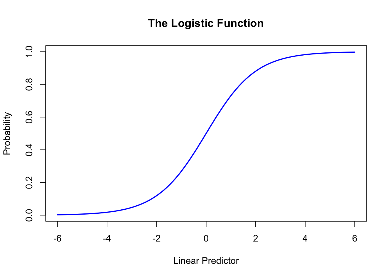
29.5 Logistic Regression

Logistic regression models binary outcomes. The response is 0 or 1 (failure or success), and we model the probability of success as a function of predictors.

The logistic function maps the linear predictor to probabilities:

\[P(Y = 1 | X) = \frac{1}{1 + e^{-(\beta_0 + \beta_1 X)}}\]

Equivalently, we model the log-odds:

\[\log\left(\frac{P}{1-P}\right) = \beta_0 + \beta_1 X\]

Code

# The logistic function
curve(1 / (1 + exp(-x)), from = -6, to = 6, 
      xlab = "Linear Predictor", ylab = "Probability",
      main = "The Logistic Function", lwd = 2, col = "blue")

Figure 29.2: The logistic function mapping the linear predictor to probabilities between 0 and 1

29.6 Fitting Logistic Regression

Code

# Example: predicting transmission type from mpg
data(mtcars)
mtcars$am <- factor(mtcars$am, labels = c("automatic", "manual"))

logit_model <- glm(am ~ mpg, data = mtcars, family = binomial)
summary(logit_model)


Call:
glm(formula = am ~ mpg, family = binomial, data = mtcars)

Coefficients:
            Estimate Std. Error z value Pr(>|z|)   
(Intercept)  -6.6035     2.3514  -2.808  0.00498 **
mpg           0.3070     0.1148   2.673  0.00751 **
---
Signif. codes:  0 '***' 0.001 '**' 0.01 '*' 0.05 '.' 0.1 ' ' 1

(Dispersion parameter for binomial family taken to be 1)

    Null deviance: 43.230  on 31  degrees of freedom
Residual deviance: 29.675  on 30  degrees of freedom
AIC: 33.675

Number of Fisher Scoring iterations: 5

29.7 Interpreting Logistic Coefficients

Coefficients are on the log-odds scale. To interpret them:

Exponentiate to get odds ratios:

Code

exp(coef(logit_model))

(Intercept)         mpg 
0.001355579 1.359379288

The odds ratio for mpg (1.36) means that each additional mpg is associated with 36% higher odds of having a manual transmission.

29.8 Making Predictions

Code

# Predict probability for specific mpg values
new_data <- data.frame(mpg = c(15, 20, 25, 30))
predict(logit_model, newdata = new_data, type = "response")

        1         2         3         4 
0.1194021 0.3862832 0.7450109 0.9313311

The type = "response" argument returns probabilities rather than log-odds.

29.9 Multiple Logistic Regression

Like linear regression, logistic regression can include multiple predictors. This allows us to:

Control for confounding variables
Examine how multiple factors together predict the outcome
Test for interactions between predictors

Code

# Multiple logistic regression: am ~ mpg + wt + hp
multi_logit <- glm(am ~ mpg + wt + hp, data = mtcars, family = binomial)
summary(multi_logit)


Call:
glm(formula = am ~ mpg + wt + hp, family = binomial, data = mtcars)

Coefficients:
             Estimate Std. Error z value Pr(>|z|)  
(Intercept) -15.72137   40.00281  -0.393   0.6943  
mpg           1.22930    1.58109   0.778   0.4369  
wt           -6.95492    3.35297  -2.074   0.0381 *
hp            0.08389    0.08228   1.020   0.3079  
---
Signif. codes:  0 '***' 0.001 '**' 0.01 '*' 0.05 '.' 0.1 ' ' 1

(Dispersion parameter for binomial family taken to be 1)

    Null deviance: 43.2297  on 31  degrees of freedom
Residual deviance:  8.7661  on 28  degrees of freedom
AIC: 16.766

Number of Fisher Scoring iterations: 10

Code

# Odds ratios for all predictors
exp(coef(multi_logit))

 (Intercept)          mpg           wt           hp 
1.486947e-07 3.418843e+00 9.539266e-04 1.087513e+00

Notice how coefficients change compared to the simple model—this is the effect of controlling for other variables.

Code

# Compare models with likelihood ratio test
anova(logit_model, multi_logit, test = "Chisq")

Analysis of Deviance Table

Model 1: am ~ mpg
Model 2: am ~ mpg + wt + hp
  Resid. Df Resid. Dev Df Deviance  Pr(>Chi)    
1        30    29.6752                          
2        28     8.7661  2   20.909 2.882e-05 ***
---
Signif. codes:  0 '***' 0.001 '**' 0.01 '*' 0.05 '.' 0.1 ' ' 1

The likelihood ratio test compares nested models. A significant p-value indicates the fuller model fits significantly better.

29.10 Poisson Regression

Poisson regression models count data—the number of events in a fixed period or area. The response must be non-negative integers, and we assume events occur independently at a constant rate.

\[\log(\mu) = \beta_0 + \beta_1 X\]

Code

# Example: modeling count data
set.seed(42)
exposure <- runif(100, 1, 10)
counts <- rpois(100, lambda = exp(0.5 + 0.3 * exposure))

pois_model <- glm(counts ~ exposure, family = poisson)
summary(pois_model)


Call:
glm(formula = counts ~ exposure, family = poisson)

Coefficients:
            Estimate Std. Error z value Pr(>|z|)    
(Intercept)  0.42499    0.10624    4.00 6.32e-05 ***
exposure     0.30714    0.01345   22.84  < 2e-16 ***
---
Signif. codes:  0 '***' 0.001 '**' 0.01 '*' 0.05 '.' 0.1 ' ' 1

(Dispersion parameter for poisson family taken to be 1)

    Null deviance: 744.110  on 99  degrees of freedom
Residual deviance:  97.826  on 98  degrees of freedom
AIC: 498.52

Number of Fisher Scoring iterations: 4

29.11 Overdispersion

A key assumption of Poisson regression is that the mean equals the variance. When variance exceeds the mean (overdispersion), standard errors are underestimated and p-values become too small.

Code

# Check for overdispersion
# Ratio of residual deviance to df should be near 1
dispersion_ratio <- pois_model$deviance / pois_model$df.residual
cat("Dispersion ratio:", round(dispersion_ratio, 3), "\n")

Dispersion ratio: 0.998

Code

cat("Values > 1.5 suggest overdispersion\n")

Values > 1.5 suggest overdispersion

Handling Overdispersion

Quasi-Poisson estimates the dispersion parameter from the data rather than assuming it equals 1:

Code

# Create overdispersed data for demonstration
set.seed(42)
n <- 100
x <- runif(n, 1, 10)
# Generate overdispersed counts (negative binomial acts like overdispersed Poisson)
y_overdispersed <- rnbinom(n, size = 2, mu = exp(0.5 + 0.3 * x))

# Standard Poisson (ignores overdispersion)
pois_fit <- glm(y_overdispersed ~ x, family = poisson)

# Quasi-Poisson (accounts for overdispersion)
quasi_fit <- glm(y_overdispersed ~ x, family = quasipoisson)

# Compare standard errors
cat("Poisson SE:", round(summary(pois_fit)$coefficients[2, 2], 4), "\n")

Poisson SE: 0.0129

Code

cat("Quasi-Poisson SE:", round(summary(quasi_fit)$coefficients[2, 2], 4), "\n")

Quasi-Poisson SE: 0.0327

Code

cat("SE inflation factor:", round(summary(quasi_fit)$coefficients[2, 2] /
                                   summary(pois_fit)$coefficients[2, 2], 2), "\n")

SE inflation factor: 2.53

Similarly, quasibinomial handles overdispersion in binomial data:

Code

# Quasibinomial example
# family = quasibinomial adjusts for extra-binomial variation

When to Use Quasi-Likelihood

Use quasipoisson or quasibinomial when:

Dispersion ratio is substantially > 1 (overdispersion)
You don’t need AIC for model comparison (quasi-models don’t have AIC)
The basic model structure is correct but variance assumptions are violated

For severe overdispersion, consider negative binomial regression (package MASS) which models overdispersion explicitly.

29.12 Model Assessment

GLMs use deviance rather than R² to assess fit. Deviance compares the fitted model to a saturated model (one parameter per observation).

Null deviance: Deviance with only the intercept Residual deviance: Deviance of the fitted model

A large drop from null to residual deviance indicates the predictors explain substantial variation.

Code

# Compare deviances
with(logit_model, null.deviance - deviance)

[1] 13.55457

Code

# Chi-square test for improvement
with(logit_model, pchisq(null.deviance - deviance, 
                         df.null - df.residual, 
                         lower.tail = FALSE))

[1] 0.0002317271

29.13 Model Comparison with AIC

As with linear models, AIC helps compare GLMs:

Code

# Compare models
model1 <- glm(am ~ mpg, data = mtcars, family = binomial)
model2 <- glm(am ~ mpg + wt, data = mtcars, family = binomial)
model3 <- glm(am ~ mpg * wt, data = mtcars, family = binomial)

AIC(model1, model2, model3)

       df      AIC
model1  2 33.67517
model2  3 23.18426
model3  4 24.49947

29.14 Assumptions and Diagnostics

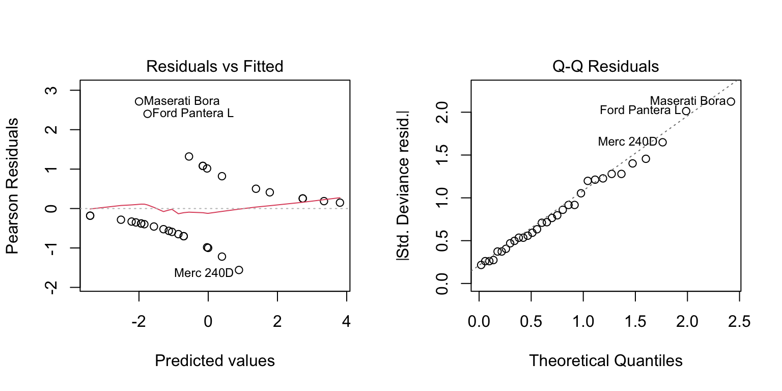
GLM assumptions include: - Correct specification of the distribution - Correct link function - Independence of observations - No extreme multicollinearity

Diagnostic tools include: - Residual plots (deviance or Pearson residuals) - Influence measures - Goodness-of-fit tests

Code

par(mfrow = c(1, 2))
plot(logit_model, which = c(1, 2))

Figure 29.3: Diagnostic plots for assessing logistic regression model assumptions

29.15 Summary

GLMs provide a flexible framework for modeling non-normal response variables while maintaining the interpretability of linear models. Logistic regression for binary outcomes and Poisson regression for counts are the most common applications, but the framework extends to other distributions as needed.

29.16 Exercises

Exercise G.1: Logistic Regression for Binary Outcomes

You study the effect of study time on exam success. Students either pass (1) or fail (0), and you record their study hours:

study_hours <- c(1, 2, 3, 4, 5, 6, 7, 8, 9, 10, 11, 12)
pass <- c(0, 0, 0, 1, 0, 1, 1, 1, 1, 1, 1, 1)

Fit a logistic regression model predicting pass/fail from study hours
Interpret the coefficient for study hours on the log-odds scale
Calculate and interpret the odds ratio for a one-hour increase in study time
Predict the probability of passing for a student who studies 5 hours
At what study time does the model predict a 50% probability of passing?
Create a visualization showing the fitted logistic curve with the observed data points

Code

# Your code here

Exercise G.2: Poisson Regression for Count Data

You count the number of bacterial colonies on petri dishes as a function of antibiotic concentration:

concentration <- c(0, 0.5, 1.0, 1.5, 2.0, 2.5, 3.0)
colonies <- c(142, 118, 89, 67, 45, 32, 21)

Fit a Poisson regression model
Interpret the coefficient for concentration
Calculate the expected number of colonies at concentration = 1.5
Check for overdispersion by comparing residual deviance to degrees of freedom
If overdispersed, refit using quasipoisson and compare standard errors
Create a plot showing observed counts and model predictions

Code

# Your code here

Exercise G.3: Model Comparison and Selection

Using the mtcars dataset, predict whether a car has an automatic transmission (am: 0 = automatic, 1 = manual) from various predictors:

Fit three logistic regression models:
- Model 1: am ~ mpg
- Model 2: am ~ mpg + wt
- Model 3: am ~ mpg + wt + hp
Compare models using AIC
Perform likelihood ratio tests to compare nested models
Which model would you choose and why?
For your chosen model, interpret the coefficients in terms of odds ratios
Use the model to predict transmission type for a car with mpg=20, wt=3.0, hp=150

Code

# Your code here

Exercise G.4: Chi-Square and Contingency Tables

A genetics study crosses two heterozygous plants and observes offspring phenotypes. Expected ratio is 9:3:3:1.

observed <- c(293, 105, 98, 32)  # Four phenotype categories

Perform a chi-square goodness-of-fit test
Calculate the expected counts and verify the chi-square assumption is met
Calculate the contribution of each category to the total chi-square statistic
Visualize observed vs. expected with a barplot
Do the data support the Mendelian hypothesis?

Now consider a 2×2 contingency table for treatment outcome by gender:

	Success	Failure
Male	45	25
Female	60	20

Test for independence using chi-square
Calculate and interpret the odds ratio
Use Fisher’s exact test and compare to the chi-square result

Code

# Your code here

Exercise G.5: Handling Overdispersion

Simulate overdispersed count data and explore the consequences:

set.seed(123)
x <- seq(1, 10, length.out = 50)
# Negative binomial creates overdispersion
y <- rnbinom(50, size = 2, mu = exp(1 + 0.3 * x))

Fit both a Poisson and quasi-Poisson model
Calculate the dispersion parameter
Compare the standard errors between the two models
How does ignoring overdispersion affect inference?
Fit a negative binomial model using MASS::glm.nb() and compare to the quasi-Poisson approach
Which model would you prefer for these data and why?

Code

# Your code here
library(MASS)  # for glm.nb()

# Generalized Linear Models {#sec-glm} ```{r} #| echo: false #| message: false library(tidyverse) theme_set(theme_minimal()) ``` ## Beyond Normal Distributions Standard linear regression assumes that the response variable is continuous and normally distributed. But many important response variables violate these assumptions. Binary outcomes (success/failure, alive/dead) follow binomial distributions. Count data (number of events, cells, species) often follow Poisson distributions. Generalized Linear Models (GLMs) extend linear regression to handle these situations. They provide a unified framework for modeling responses that follow different distributions from the exponential family. ## Frequency Analysis: Categorical Response Variables Before diving into GLMs, it's important to understand how we analyze categorical response variables. When observations fall into categories rather than being measured on a continuous scale, we count the frequency in each category and compare observed frequencies to expected values. ### Chi-Square Goodness of Fit Test The **goodness of fit test** asks whether observed frequencies match a hypothesized distribution. The classic example comes from Mendelian genetics. ```{r} # Mendel's pea experiment - F2 phenotype ratios # Expected: 9:3:3:1 for Yellow-Smooth:Yellow-Wrinkled:Green-Smooth:Green-Wrinkled observed <- c(315, 101, 108, 32) # Mendel's actual data expected_ratios <- c(9/16, 3/16, 3/16, 1/16) # Perform chi-square test chisq.test(observed, p = expected_ratios) ``` The test statistic measures deviation from expected: $$\chi^2 = \sum \frac{(O_i - E_i)^2}{E_i}$$ where $O_i$ are observed and $E_i$ are expected counts. Under the null hypothesis (observed frequencies match expected), this follows a chi-square distribution with $df = k - 1$ where $k$ is the number of categories. ::: {.callout-warning} ## Chi-Square Assumptions 1. **Independence**: Observations must be independent 2. **Expected counts**: No more than 20% of expected counts should be < 5 3. **Sample size**: Total sample should be reasonably large Check expected values before interpreting results: ```{r} n <- sum(observed) expected <- n * expected_ratios cat("Expected counts:", round(expected, 1)) ``` ::: ### Contingency Table Analysis When we have two categorical variables, we use a **contingency table** to examine their association. The null hypothesis is that the variables are independent. ```{r} # Example: Hair color and eye color association # Data from 1000 students hair_eye <- matrix(c(347, 191, # Blue eyes: blonde, brunette 177, 329), # Brown eyes: blonde, brunette nrow = 2, byrow = TRUE) rownames(hair_eye) <- c("Blue_eyes", "Brown_eyes") colnames(hair_eye) <- c("Blonde", "Brunette") # View the contingency table hair_eye # Chi-square test of independence chisq.test(hair_eye) ``` For contingency tables, $df = (r-1)(c-1)$ where $r$ and $c$ are the number of rows and columns. ```{r} #| label: fig-mosaic-plot #| fig-cap: "Mosaic plot showing the association between hair color and eye color" #| fig-width: 7 #| fig-height: 5 # Visualize with a mosaic plot mosaicplot(hair_eye, main = "Hair and Eye Color Association", color = c("gold", "brown"), shade = FALSE) ``` ### Standardized Residuals To understand where associations are strongest, examine **standardized residuals**: ```{r} # Which cells deviate most from independence? test_result <- chisq.test(hair_eye) test_result$residuals ``` Residuals > 2 or < -2 indicate cells contributing substantially to the association. Positive residuals mean more observations than expected under independence; negative means fewer. ### G-Test (Log-Likelihood Ratio Test) The **G-test** is an alternative to chi-square based on likelihood ratios: $$G = 2 \sum O_i \ln\left(\frac{O_i}{E_i}\right)$$ The G-test and chi-square give similar results for large samples, but G-tests are preferred when: - Sample sizes are small - Differences between observed and expected are small - You want to decompose complex tables ```{r} # Manual G-test calculation observed_flat <- as.vector(hair_eye) expected_flat <- as.vector(test_result$expected) G <- 2 * sum(observed_flat * log(observed_flat / expected_flat)) p_value <- 1 - pchisq(G, df = 1) cat("G statistic:", round(G, 3), "\n") cat("p-value:", format(p_value, scientific = TRUE), "\n") ``` ### Odds Ratios: Measuring Effect Size The chi-square test tells us *whether* variables are associated, but not the **strength** of association. For 2×2 tables, the **odds ratio** quantifies effect size. The odds of an event are $\frac{p}{1-p}$. The odds ratio compares odds between groups: $$OR = \frac{odds_1}{odds_2} = \frac{a/b}{c/d} = \frac{ad}{bc}$$ ```{r} # Odds ratio for hair/eye color data a <- hair_eye[1,1] # Blue eyes, Blonde b <- hair_eye[1,2] # Blue eyes, Brunette c <- hair_eye[2,1] # Brown eyes, Blonde d <- hair_eye[2,2] # Brown eyes, Brunette odds_ratio <- (a * d) / (b * c) cat("Odds Ratio:", round(odds_ratio, 2), "\n") ``` An OR of `r round(odds_ratio, 2)` means blue-eyed individuals have about `r round(odds_ratio, 1)` times the odds of being blonde compared to brown-eyed individuals. - OR = 1: No association - OR > 1: Positive association - OR < 1: Negative association ```{r} # Confidence interval for odds ratio (using log transform) log_OR <- log(odds_ratio) se_log_OR <- sqrt(1/a + 1/b + 1/c + 1/d) ci_log <- log_OR + c(-1.96, 1.96) * se_log_OR ci_OR <- exp(ci_log) cat("95% CI for OR: [", round(ci_OR[1], 2), ",", round(ci_OR[2], 2), "]\n") ``` ### Fisher's Exact Test For small sample sizes (expected counts < 5), **Fisher's exact test** is more appropriate. It calculates exact probabilities rather than relying on the chi-square approximation. ```{r} # Small sample example small_table <- matrix(c(3, 1, 1, 3), nrow = 2) fisher.test(small_table) ``` Fisher's test is preferred for 2×2 tables with small samples and provides a confidence interval for the odds ratio. ## Components of a GLM GLMs have three components: **Random component**: Specifies the probability distribution of the response variable (e.g., binomial, Poisson, normal). **Systematic component**: The linear predictor, a linear combination of explanatory variables: $$\eta = \beta_0 + \beta_1 x_1 + \beta_2 x_2 + \ldots$$ **Link function**: Connects the random and systematic components, transforming the expected value of the response to the scale of the linear predictor. ## The Link Function Different distributions use different link functions: | Distribution | Typical Link | Link Function | |:-------------|:-------------|:--------------| | Normal | Identity | $\eta = \mu$ | | Binomial | Logit | $\eta = \log(\frac{\mu}{1-\mu})$ | | Poisson | Log | $\eta = \log(\mu)$ | ## Logistic Regression Logistic regression models binary outcomes. The response is 0 or 1 (failure or success), and we model the probability of success as a function of predictors. The logistic function maps the linear predictor to probabilities: $$P(Y = 1 | X) = \frac{1}{1 + e^{-(\beta_0 + \beta_1 X)}}$$ Equivalently, we model the log-odds: $$\log\left(\frac{P}{1-P}\right) = \beta_0 + \beta_1 X$$ ```{r} #| label: fig-logistic-function #| fig-cap: "The logistic function mapping the linear predictor to probabilities between 0 and 1" #| fig-width: 7 #| fig-height: 5 # The logistic function curve(1 / (1 + exp(-x)), from = -6, to = 6, xlab = "Linear Predictor", ylab = "Probability", main = "The Logistic Function", lwd = 2, col = "blue") ``` ## Fitting Logistic Regression ```{r} # Example: predicting transmission type from mpg data(mtcars) mtcars$am <- factor(mtcars$am, labels = c("automatic", "manual")) logit_model <- glm(am ~ mpg, data = mtcars, family = binomial) summary(logit_model) ``` ## Interpreting Logistic Coefficients Coefficients are on the log-odds scale. To interpret them: **Exponentiate** to get odds ratios: ```{r} exp(coef(logit_model)) ``` The odds ratio for mpg (1.36) means that each additional mpg is associated with 36% higher odds of having a manual transmission. ## Making Predictions ```{r} # Predict probability for specific mpg values new_data <- data.frame(mpg = c(15, 20, 25, 30)) predict(logit_model, newdata = new_data, type = "response") ``` The `type = "response"` argument returns probabilities rather than log-odds. ## Multiple Logistic Regression Like linear regression, logistic regression can include multiple predictors. This allows us to: - Control for confounding variables - Examine how multiple factors together predict the outcome - Test for interactions between predictors ```{r} # Multiple logistic regression: am ~ mpg + wt + hp multi_logit <- glm(am ~ mpg + wt + hp, data = mtcars, family = binomial) summary(multi_logit) ``` ```{r} # Odds ratios for all predictors exp(coef(multi_logit)) ``` Notice how coefficients change compared to the simple model—this is the effect of controlling for other variables. ```{r} # Compare models with likelihood ratio test anova(logit_model, multi_logit, test = "Chisq") ``` The likelihood ratio test compares nested models. A significant p-value indicates the fuller model fits significantly better. ## Poisson Regression Poisson regression models count data—the number of events in a fixed period or area. The response must be non-negative integers, and we assume events occur independently at a constant rate. $$\log(\mu) = \beta_0 + \beta_1 X$$ ```{r} # Example: modeling count data set.seed(42) exposure <- runif(100, 1, 10) counts <- rpois(100, lambda = exp(0.5 + 0.3 * exposure)) pois_model <- glm(counts ~ exposure, family = poisson) summary(pois_model) ``` ## Overdispersion A key assumption of Poisson regression is that the mean equals the variance. When variance exceeds the mean (**overdispersion**), standard errors are underestimated and p-values become too small. ```{r} # Check for overdispersion # Ratio of residual deviance to df should be near 1 dispersion_ratio <- pois_model$deviance / pois_model$df.residual cat("Dispersion ratio:", round(dispersion_ratio, 3), "\n") cat("Values > 1.5 suggest overdispersion\n") ``` ### Handling Overdispersion **Quasi-Poisson** estimates the dispersion parameter from the data rather than assuming it equals 1: ```{r} # Create overdispersed data for demonstration set.seed(42) n <- 100 x <- runif(n, 1, 10) # Generate overdispersed counts (negative binomial acts like overdispersed Poisson) y_overdispersed <- rnbinom(n, size = 2, mu = exp(0.5 + 0.3 * x)) # Standard Poisson (ignores overdispersion) pois_fit <- glm(y_overdispersed ~ x, family = poisson) # Quasi-Poisson (accounts for overdispersion) quasi_fit <- glm(y_overdispersed ~ x, family = quasipoisson) # Compare standard errors cat("Poisson SE:", round(summary(pois_fit)$coefficients[2, 2], 4), "\n") cat("Quasi-Poisson SE:", round(summary(quasi_fit)$coefficients[2, 2], 4), "\n") cat("SE inflation factor:", round(summary(quasi_fit)$coefficients[2, 2] / summary(pois_fit)$coefficients[2, 2], 2), "\n") ``` Similarly, **quasibinomial** handles overdispersion in binomial data: ```{r} # Quasibinomial example # family = quasibinomial adjusts for extra-binomial variation ``` ::: {.callout-tip} ## When to Use Quasi-Likelihood Use `quasipoisson` or `quasibinomial` when: - Dispersion ratio is substantially > 1 (overdispersion) - You don't need AIC for model comparison (quasi-models don't have AIC) - The basic model structure is correct but variance assumptions are violated For severe overdispersion, consider **negative binomial regression** (package `MASS`) which models overdispersion explicitly. ::: ## Model Assessment GLMs use **deviance** rather than R² to assess fit. Deviance compares the fitted model to a saturated model (one parameter per observation). **Null deviance**: Deviance with only the intercept **Residual deviance**: Deviance of the fitted model A large drop from null to residual deviance indicates the predictors explain substantial variation. ```{r} # Compare deviances with(logit_model, null.deviance - deviance) # Chi-square test for improvement with(logit_model, pchisq(null.deviance - deviance, df.null - df.residual, lower.tail = FALSE)) ``` ## Model Comparison with AIC As with linear models, AIC helps compare GLMs: ```{r} # Compare models model1 <- glm(am ~ mpg, data = mtcars, family = binomial) model2 <- glm(am ~ mpg + wt, data = mtcars, family = binomial) model3 <- glm(am ~ mpg * wt, data = mtcars, family = binomial) AIC(model1, model2, model3) ``` ## Assumptions and Diagnostics GLM assumptions include: - Correct specification of the distribution - Correct link function - Independence of observations - No extreme multicollinearity Diagnostic tools include: - Residual plots (deviance or Pearson residuals) - Influence measures - Goodness-of-fit tests ```{r} #| label: fig-glm-diagnostics #| fig-cap: "Diagnostic plots for assessing logistic regression model assumptions" #| fig-width: 8 #| fig-height: 4 par(mfrow = c(1, 2)) plot(logit_model, which = c(1, 2)) ``` ## Summary GLMs provide a flexible framework for modeling non-normal response variables while maintaining the interpretability of linear models. Logistic regression for binary outcomes and Poisson regression for counts are the most common applications, but the framework extends to other distributions as needed. ## Exercises ::: {.callout-note} ### Exercise G.1: Logistic Regression for Binary Outcomes You study the effect of study time on exam success. Students either pass (1) or fail (0), and you record their study hours: ``` study_hours <- c(1, 2, 3, 4, 5, 6, 7, 8, 9, 10, 11, 12) pass <- c(0, 0, 0, 1, 0, 1, 1, 1, 1, 1, 1, 1) ``` a) Fit a logistic regression model predicting pass/fail from study hours b) Interpret the coefficient for study hours on the log-odds scale c) Calculate and interpret the odds ratio for a one-hour increase in study time d) Predict the probability of passing for a student who studies 5 hours e) At what study time does the model predict a 50% probability of passing? f) Create a visualization showing the fitted logistic curve with the observed data points ```{r} #| eval: false # Your code here ``` ::: ::: {.callout-note} ### Exercise G.2: Poisson Regression for Count Data You count the number of bacterial colonies on petri dishes as a function of antibiotic concentration: ``` concentration <- c(0, 0.5, 1.0, 1.5, 2.0, 2.5, 3.0) colonies <- c(142, 118, 89, 67, 45, 32, 21) ``` a) Fit a Poisson regression model b) Interpret the coefficient for concentration c) Calculate the expected number of colonies at concentration = 1.5 d) Check for overdispersion by comparing residual deviance to degrees of freedom e) If overdispersed, refit using quasipoisson and compare standard errors f) Create a plot showing observed counts and model predictions ```{r} #| eval: false # Your code here ``` ::: ::: {.callout-note} ### Exercise G.3: Model Comparison and Selection Using the `mtcars` dataset, predict whether a car has an automatic transmission (`am`: 0 = automatic, 1 = manual) from various predictors: a) Fit three logistic regression models: - Model 1: `am ~ mpg` - Model 2: `am ~ mpg + wt` - Model 3: `am ~ mpg + wt + hp` b) Compare models using AIC c) Perform likelihood ratio tests to compare nested models d) Which model would you choose and why? e) For your chosen model, interpret the coefficients in terms of odds ratios f) Use the model to predict transmission type for a car with mpg=20, wt=3.0, hp=150 ```{r} #| eval: false # Your code here ``` ::: ::: {.callout-note} ### Exercise G.4: Chi-Square and Contingency Tables A genetics study crosses two heterozygous plants and observes offspring phenotypes. Expected ratio is 9:3:3:1. ``` observed <- c(293, 105, 98, 32) # Four phenotype categories ``` a) Perform a chi-square goodness-of-fit test b) Calculate the expected counts and verify the chi-square assumption is met c) Calculate the contribution of each category to the total chi-square statistic d) Visualize observed vs. expected with a barplot e) Do the data support the Mendelian hypothesis? Now consider a 2×2 contingency table for treatment outcome by gender: | | Success | Failure | |:--|:--------|:--------| | Male | 45 | 25 | | Female | 60 | 20 | f) Test for independence using chi-square g) Calculate and interpret the odds ratio h) Use Fisher's exact test and compare to the chi-square result ```{r} #| eval: false # Your code here ``` ::: ::: {.callout-note} ### Exercise G.5: Handling Overdispersion Simulate overdispersed count data and explore the consequences: ``` set.seed(123) x <- seq(1, 10, length.out = 50) # Negative binomial creates overdispersion y <- rnbinom(50, size = 2, mu = exp(1 + 0.3 * x)) ``` a) Fit both a Poisson and quasi-Poisson model b) Calculate the dispersion parameter c) Compare the standard errors between the two models d) How does ignoring overdispersion affect inference? e) Fit a negative binomial model using `MASS::glm.nb()` and compare to the quasi-Poisson approach f) Which model would you prefer for these data and why? ```{r} #| eval: false # Your code here library(MASS) # for glm.nb() ``` :::