Power is the probability of correctly rejecting a false null hypothesis—the probability of detecting an effect when one truly exists. If the true effect size is non-zero, power tells us how likely our study is to find it.
Power = 1 - \(\beta\), where \(\beta\) is the probability of a Type II error (failing to reject a false null hypothesis). We typically aim for power of at least 80%, meaning we accept a 20% chance of missing a true effect.
Figure 25.1: Illustration of statistical power showing the relationship between Type I error (alpha), Type II error (beta), and power in hypothesis testing
25.2 Why Power Matters
A study with low power has poor chances of detecting true effects. Even if an effect exists, the study may fail to find statistical significance. Worse, significant results from underpowered studies tend to overestimate effect sizes—a phenomenon called the “winner’s curse.”
Understanding power helps us interpret results appropriately. If we fail to reject the null hypothesis, was it because no effect exists, or because our study lacked the power to detect it?
25.3 Determinants of Power
Power depends on four factors that are mathematically related:
Effect Size: Larger effects are easier to detect. Effect size can be measured in original units or standardized (like Cohen’s d).
Sample Size (n): Larger samples provide more information and higher power.
Significance Level (\(\alpha\)): Using a more lenient alpha (e.g., 0.10 instead of 0.05) increases power but also increases Type I error risk.
Variability (\(\sigma\)): Less variable data makes effects easier to detect.
Figure 25.2: Visual representation of the four factors that determine statistical power: effect size, sample size, significance level, and variability
25.4 Cohen’s d: Standardized Effect Size
Cohen’s d expresses the difference between means in standard deviation units:
\[d = \frac{\mu_1 - \mu_2}{s_{pooled}}\]
Conventional benchmarks (Cohen, 1988): - d = 0.2: small effect - d = 0.5: medium effect - d = 0.8: large effect
These benchmarks are only guidelines—what counts as “small” depends on the research context.
25.5 A Priori Power Analysis
Before collecting data, power analysis helps determine the sample size needed to detect effects of interest. This requires specifying:
The expected effect size
The desired power (typically 0.80)
The significance level (typically 0.05)
The statistical test to be used
Code
# How many subjects needed to detect d = 0.5 with 80% power?pwr.t.test(d =0.5, sig.level =0.05, power =0.80, type ="two.sample")
     Two-sample t test power calculation

              n = 63.76561
              d = 0.5
      sig.level = 0.05
          power = 0.8
    alternative = two.sided

NOTE: n is number in *each* group
About 64 subjects per group are needed to detect a medium effect with 80% power using a two-sample t-test.
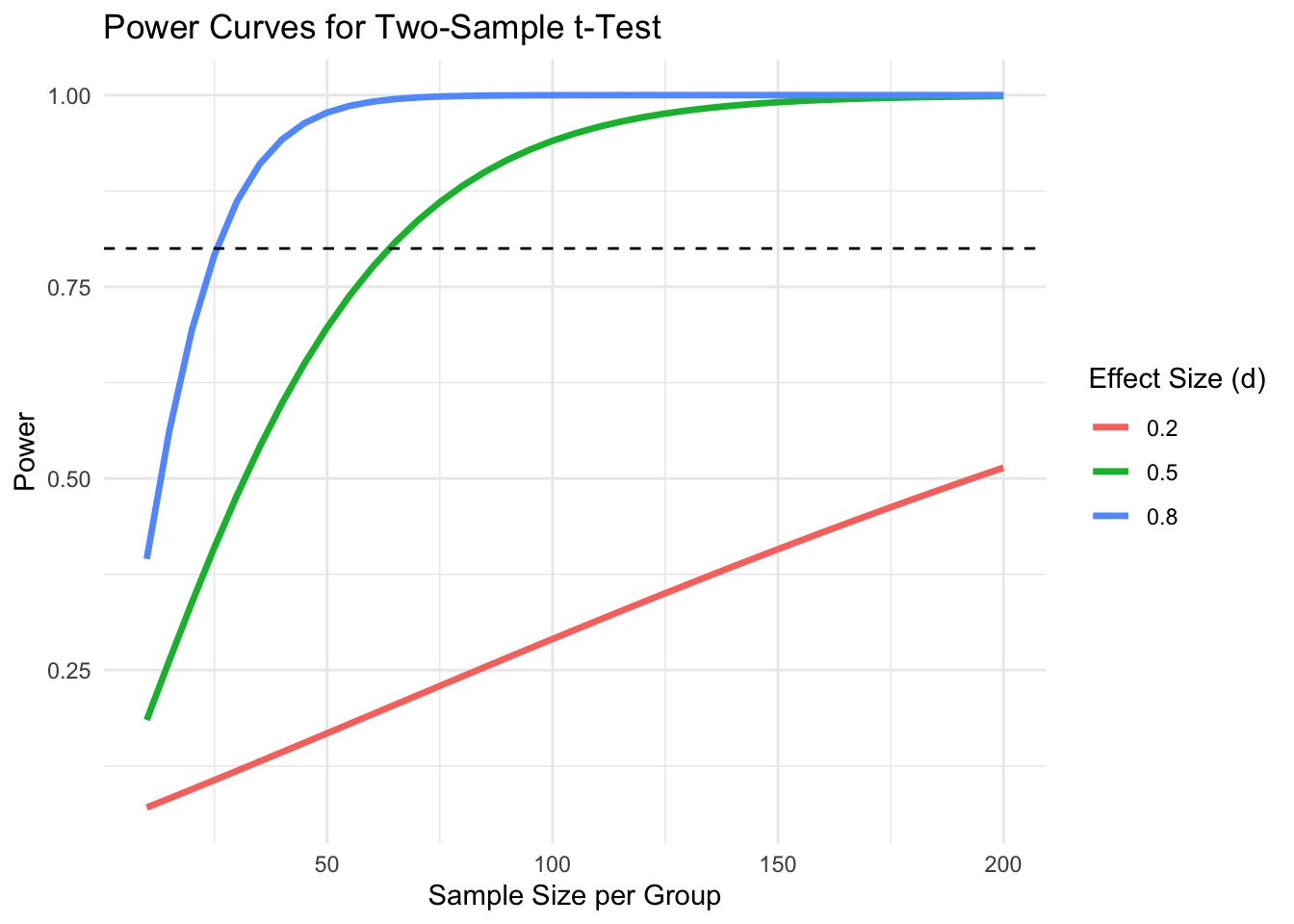
25.6 Power Curves
Power curves show how power changes with sample size or effect size:
Code
# Power curve for different effect sizessample_sizes <-seq(10, 200, by =5)effect_sizes <-c(0.2, 0.5, 0.8)power_data <-expand.grid(n = sample_sizes, d = effect_sizes)power_data$power <-mapply(function(n, d) {pwr.t.test(n = n, d = d, sig.level =0.05, type ="two.sample")$power}, power_data$n, power_data$d)ggplot(power_data, aes(x = n, y = power, color =factor(d))) +geom_line(size =1.2) +geom_hline(yintercept =0.8, linetype ="dashed") +labs(title ="Power Curves for Two-Sample t-Test",x ="Sample Size per Group",y ="Power",color ="Effect Size (d)") +theme_minimal()
Figure 25.3: Power curves showing how statistical power increases with sample size for different effect sizes (Cohen’s d = 0.2, 0.5, 0.8) in a two-sample t-test
25.7 Power for ANOVA
For ANOVA, effect size is measured by Cohen’s f:
\[f = \frac{\sigma_{between}}{\sigma_{within}}\]
Benchmarks: f = 0.10 (small), f = 0.25 (medium), f = 0.40 (large).
Code
# Sample size for ANOVA with 3 groupspwr.anova.test(k =3, f =0.25, sig.level =0.05, power =0.80)
     Balanced one-way analysis of variance power calculation

              k = 3
              n = 52.3966
              f = 0.25
      sig.level = 0.05
          power = 0.8

NOTE: n is number in each group
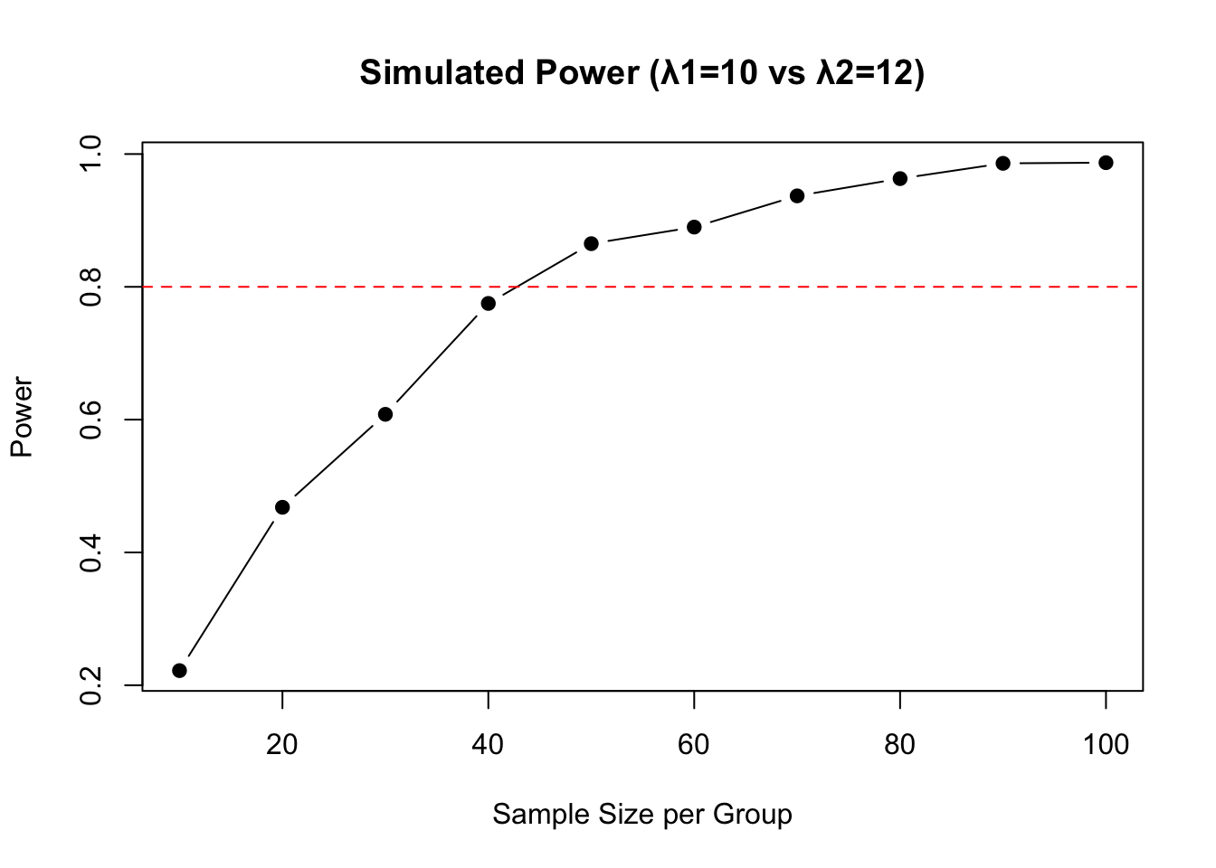
25.8 Simulation-Based Power Analysis
For complex designs, simulation provides a flexible approach:
Code
# Simulation-based power for comparing two Poisson distributionsset.seed(42)power_sim <-function(n, lambda1, lambda2, n_sims =1000) { significant <-replicate(n_sims, { x1 <-rpois(n, lambda1) x2 <-rpois(n, lambda2)t.test(x1, x2)$p.value <0.05 })mean(significant)}# Power for different sample sizessample_sizes <-seq(10, 100, by =10)powers <-sapply(sample_sizes, power_sim, lambda1 =10, lambda2 =12)plot(sample_sizes, powers, type ="b", pch =19,xlab ="Sample Size per Group", ylab ="Power",main ="Simulated Power (λ1=10 vs λ2=12)")abline(h =0.8, lty =2, col ="red")
Figure 25.4: Simulation-based power analysis for comparing two Poisson distributions, showing power as a function of sample size
25.9 Post Hoc Power Analysis
Calculating power after a study is completed is controversial. Post hoc power calculated from observed effect sizes is mathematically determined by the p-value and adds no new information. It cannot tell you whether a non-significant result reflects a true null or insufficient power.
If you want to understand what your study could detect, specify effect sizes based on scientific considerations, not observed results.
25.10 Practical Recommendations
Always conduct power analysis before data collection. Use realistic effect size estimates based on pilot data or previous literature. Consider what effect size would be practically meaningful, not just what you think exists.
Be conservative—effects are often smaller than expected. Plan for some attrition or missing data. When in doubt, collect more data if feasible.
Source Code
# Statistical Power {#sec-power}```{r}#| echo: false#| message: falselibrary(tidyverse)library(pwr)theme_set(theme_minimal())```## What is Statistical Power?Power is the probability of correctly rejecting a false null hypothesis—the probability of detecting an effect when one truly exists. If the true effect size is non-zero, power tells us how likely our study is to find it.Power = 1 - $\beta$, where $\beta$ is the probability of a Type II error (failing to reject a false null hypothesis). We typically aim for power of at least 80%, meaning we accept a 20% chance of missing a true effect.{#fig-power-concept fig-align="center"}## Why Power MattersA study with low power has poor chances of detecting true effects. Even if an effect exists, the study may fail to find statistical significance. Worse, significant results from underpowered studies tend to overestimate effect sizes—a phenomenon called the "winner's curse."Understanding power helps us interpret results appropriately. If we fail to reject the null hypothesis, was it because no effect exists, or because our study lacked the power to detect it?## Determinants of PowerPower depends on four factors that are mathematically related:$$\text{Power} \propto \frac{(\text{Effect Size}) \times (\alpha) \times (\sqrt{n})}{\sigma}$$**Effect Size**: Larger effects are easier to detect. Effect size can be measured in original units or standardized (like Cohen's d).**Sample Size (n)**: Larger samples provide more information and higher power.**Significance Level ($\alpha$)**: Using a more lenient alpha (e.g., 0.10 instead of 0.05) increases power but also increases Type I error risk.**Variability ($\sigma$)**: Less variable data makes effects easier to detect.{#fig-power-determinants fig-align="center"}## Cohen's d: Standardized Effect SizeCohen's d expresses the difference between means in standard deviation units:$$d = \frac{\mu_1 - \mu_2}{s_{pooled}}$$Conventional benchmarks (Cohen, 1988):- d = 0.2: small effect- d = 0.5: medium effect- d = 0.8: large effectThese benchmarks are only guidelines—what counts as "small" depends on the research context.## A Priori Power AnalysisBefore collecting data, power analysis helps determine the sample size needed to detect effects of interest. This requires specifying:1. The expected effect size2. The desired power (typically 0.80)3. The significance level (typically 0.05)4. The statistical test to be used```{r}# How many subjects needed to detect d = 0.5 with 80% power?pwr.t.test(d =0.5, sig.level =0.05, power =0.80, type ="two.sample")```About 64 subjects per group are needed to detect a medium effect with 80% power using a two-sample t-test.## Power CurvesPower curves show how power changes with sample size or effect size:```{r}#| label: fig-power-curves#| fig-cap: "Power curves showing how statistical power increases with sample size for different effect sizes (Cohen's d = 0.2, 0.5, 0.8) in a two-sample t-test"#| fig-width: 7#| fig-height: 5# Power curve for different effect sizessample_sizes <-seq(10, 200, by =5)effect_sizes <-c(0.2, 0.5, 0.8)power_data <-expand.grid(n = sample_sizes, d = effect_sizes)power_data$power <-mapply(function(n, d) {pwr.t.test(n = n, d = d, sig.level =0.05, type ="two.sample")$power}, power_data$n, power_data$d)ggplot(power_data, aes(x = n, y = power, color =factor(d))) +geom_line(size =1.2) +geom_hline(yintercept =0.8, linetype ="dashed") +labs(title ="Power Curves for Two-Sample t-Test",x ="Sample Size per Group",y ="Power",color ="Effect Size (d)") +theme_minimal()```## Power for ANOVAFor ANOVA, effect size is measured by Cohen's f:$$f = \frac{\sigma_{between}}{\sigma_{within}}$$Benchmarks: f = 0.10 (small), f = 0.25 (medium), f = 0.40 (large).```{r}# Sample size for ANOVA with 3 groupspwr.anova.test(k =3, f =0.25, sig.level =0.05, power =0.80)```## Simulation-Based Power AnalysisFor complex designs, simulation provides a flexible approach:```{r}#| label: fig-simulated-power#| fig-cap: "Simulation-based power analysis for comparing two Poisson distributions, showing power as a function of sample size"#| fig-width: 7#| fig-height: 5# Simulation-based power for comparing two Poisson distributionsset.seed(42)power_sim <-function(n, lambda1, lambda2, n_sims =1000) { significant <-replicate(n_sims, { x1 <-rpois(n, lambda1) x2 <-rpois(n, lambda2)t.test(x1, x2)$p.value <0.05 })mean(significant)}# Power for different sample sizessample_sizes <-seq(10, 100, by =10)powers <-sapply(sample_sizes, power_sim, lambda1 =10, lambda2 =12)plot(sample_sizes, powers, type ="b", pch =19,xlab ="Sample Size per Group", ylab ="Power",main ="Simulated Power (λ1=10 vs λ2=12)")abline(h =0.8, lty =2, col ="red")```## Post Hoc Power AnalysisCalculating power after a study is completed is controversial. Post hoc power calculated from observed effect sizes is mathematically determined by the p-value and adds no new information. It cannot tell you whether a non-significant result reflects a true null or insufficient power.If you want to understand what your study could detect, specify effect sizes based on scientific considerations, not observed results.## Practical RecommendationsAlways conduct power analysis before data collection. Use realistic effect size estimates based on pilot data or previous literature. Consider what effect size would be practically meaningful, not just what you think exists.Be conservative—effects are often smaller than expected. Plan for some attrition or missing data. When in doubt, collect more data if feasible.