31 Regularization Methods

31.1 The Need for Regularization

Standard linear regression estimates coefficients by minimizing the residual sum of squares (RSS):

\[\text{RSS} = \sum_{i=1}^n \left(y_i - \beta_0 - \sum_{j=1}^p \beta_j x_{ij}\right)^2\]

This works well when you have many more observations than predictors ($n \gg p$) and the predictors are not highly correlated. But problems arise in several common situations.

When you have many predictors relative to the number of observations, coefficient estimates become unstable and their variance is high. The model has too many degrees of freedom to estimate reliably from the available data. When predictors are highly correlated (multicollinearity), the problem is compounded: small changes in the data can cause dramatic swings in the estimated coefficients, even though predictions remain stable. In either case, the result is often overfitting—the model fits the training data well but predicts poorly on new observations.

Regularization addresses these issues by adding a penalty term that shrinks coefficients toward zero. This intentionally introduces a small amount of bias in exchange for a substantial reduction in variance. The net effect is usually better predictions on new data, especially when the number of predictors is large relative to the sample size.

31.2 The Regularization Idea

Regularized regression minimizes a modified objective:

\[\text{Minimize: } \text{RSS} + \lambda \cdot P(\beta)\]

In this formulation, $P(\beta)$ is a penalty function that penalizes large coefficients, and $\lambda \geq 0$ is the regularization parameter that controls the strength of the penalty.

The effect of the penalty is to shrink coefficients toward zero, with $\lambda$ controlling how aggressively. When $\lambda = 0$, there is no penalty and we recover ordinary least squares. As $\lambda$ increases, the penalty becomes stronger and coefficients shrink more. In the limit as $\lambda \to \infty$, all coefficients are forced to zero.

Different choices of the penalty function $P(\beta)$ lead to different regularization methods, each with distinct properties and use cases.

31.3 Ridge Regression (L2 Penalty)

Ridge regression (Hoerl and Kennard 1970) uses the sum of squared coefficients as the penalty:

\[P(\beta) = \sum_{j=1}^p \beta_j^2\]

The full optimization problem is:

\[\hat{\beta}^{\text{ridge}} = \arg\min_\beta \left\{ \sum_{i=1}^n \left(y_i - \beta_0 - \sum_{j=1}^p \beta_j x_{ij}\right)^2 + \lambda \sum_{j=1}^p \beta_j^2 \right\}\]

Properties of Ridge Regression

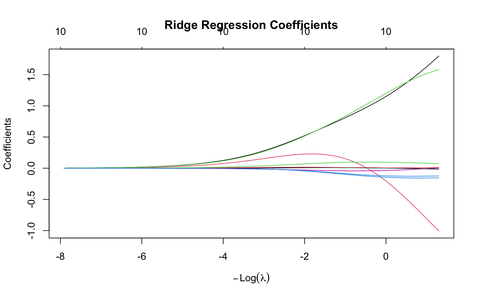
Ridge regression shrinks all coefficients toward zero but never exactly to zero. This means all predictors remain in the model regardless of how large $\lambda$ becomes—coefficients get very small but never vanish entirely. This property makes ridge regression particularly useful when you believe all predictors are relevant to some degree. It is also especially effective when predictors are highly correlated (multicollinearity), as the penalty stabilizes the coefficient estimates that would otherwise be wildly unstable in ordinary least squares.

Code

# Generate sample data with correlated predictors
set.seed(42)
n <- 100
p <- 10
X <- matrix(rnorm(n * p), n, p)
# Create correlated predictors
X[, 2] <- X[, 1] + rnorm(n, sd = 0.5)
X[, 3] <- X[, 1] + rnorm(n, sd = 0.5)
true_beta <- c(3, -2, 1.5, rep(0, p - 3))
y <- X %*% true_beta + rnorm(n)

# Fit ridge regression across lambda values
ridge_fit <- glmnet(X, y, alpha = 0)  # alpha = 0 for ridge

# Plot coefficient paths
plot(ridge_fit, xvar = "lambda", main = "Ridge Regression Coefficients")

Figure 31.1: Ridge regression coefficient paths: as lambda increases, coefficients shrink toward zero but never reach exactly zero

Geometric Interpretation

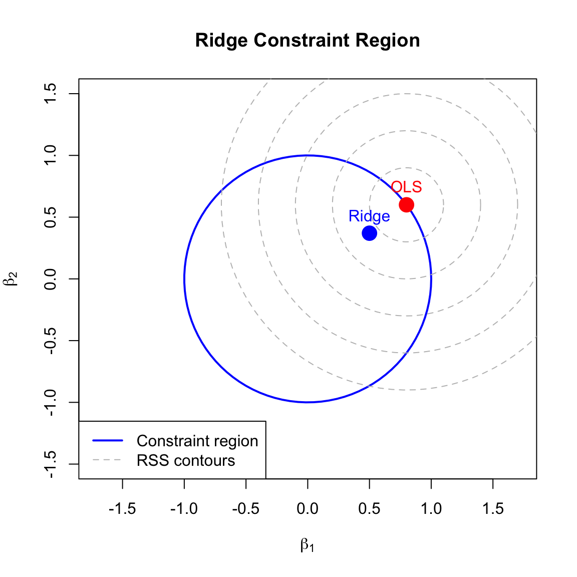
Ridge regression constrains coefficients to lie within a sphere (in 2D, a circle) centered at the origin:

\[\sum_{j=1}^p \beta_j^2 \leq t\]

where $t$ is inversely related to $\lambda$. The OLS solution may lie outside this constraint region, so ridge finds the point where the RSS contours first touch the constraint boundary.

Code

# Geometric illustration
theta <- seq(0, 2*pi, length.out = 100)

plot(cos(theta), sin(theta), type = "l", lwd = 2, col = "blue",
     asp = 1, xlim = c(-1.5, 1.5), ylim = c(-1.5, 1.5),
     xlab = expression(beta[1]), ylab = expression(beta[2]),
     main = "Ridge Constraint Region")

# Add contours representing RSS
for (r in seq(0.3, 1.5, 0.3)) {
  lines(r * cos(theta) + 0.8, r * sin(theta) + 0.6,
        col = "gray", lty = 2)
}

# OLS estimate
points(0.8, 0.6, pch = 19, cex = 2, col = "red")
text(0.8, 0.75, "OLS", col = "red")

# Ridge estimate (on boundary)
points(0.5, 0.37, pch = 19, cex = 2, col = "blue")
text(0.5, 0.5, "Ridge", col = "blue")

legend("bottomleft", c("Constraint region", "RSS contours"),
       col = c("blue", "gray"), lty = c(1, 2), lwd = c(2, 1))

Figure 31.2: Geometric interpretation of ridge regression: the constraint region is circular, so the solution rarely lies exactly on an axis (coefficient rarely zero)

31.4 Lasso Regression (L1 Penalty)

Lasso (Least Absolute Shrinkage and Selection Operator) (Tibshirani 1996) uses the sum of absolute values as the penalty:

\[P(\beta) = \sum_{j=1}^p |\beta_j|\]

The optimization problem is:

\[\hat{\beta}^{\text{lasso}} = \arg\min_\beta \left\{ \sum_{i=1}^n \left(y_i - \beta_0 - \sum_{j=1}^p \beta_j x_{ij}\right)^2 + \lambda \sum_{j=1}^p |\beta_j| \right\}\]

Properties of Lasso Regression

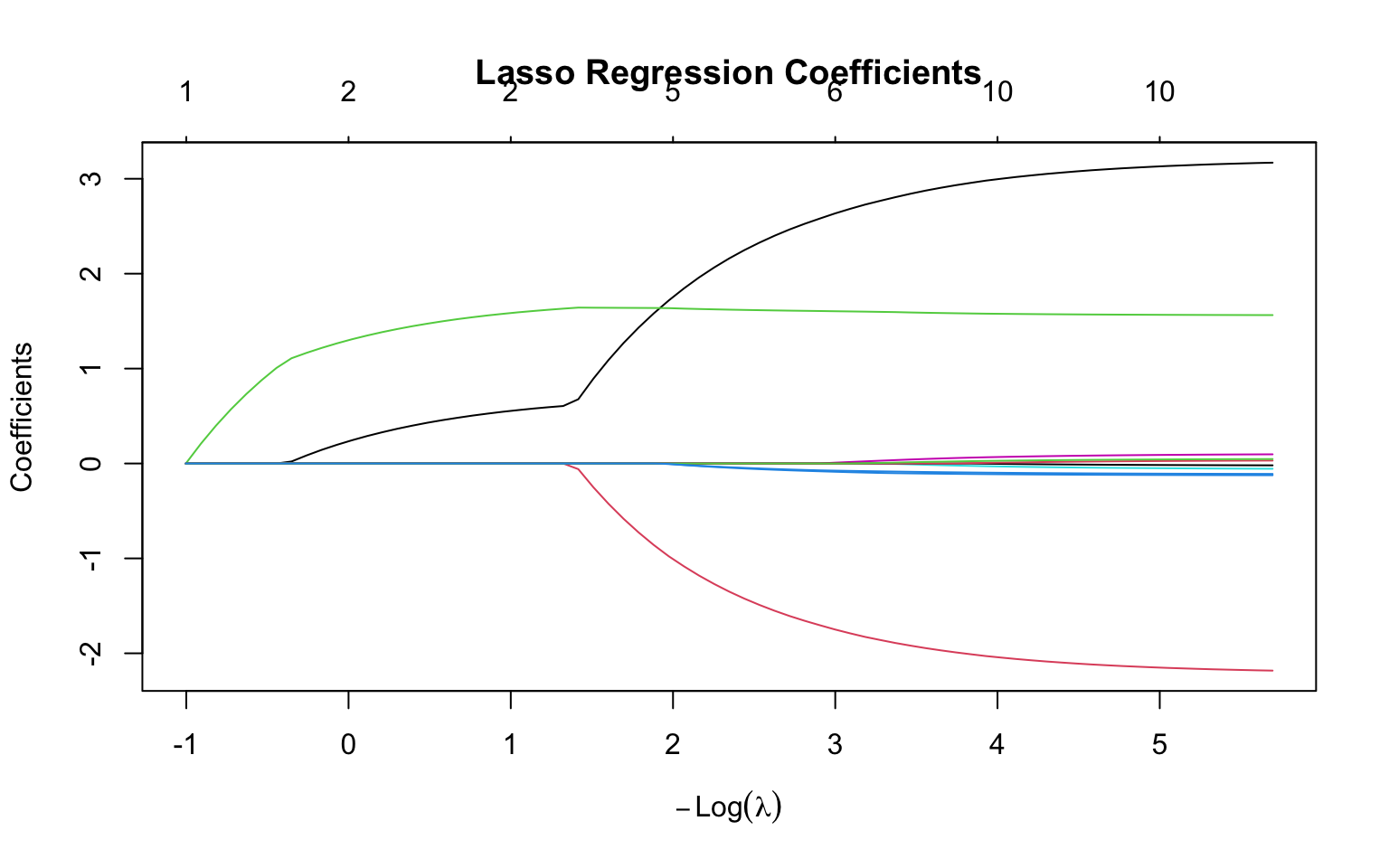
Unlike ridge, lasso can shrink coefficients exactly to zero, effectively performing variable selection. This produces sparse models with fewer predictors, making the resulting models easier to interpret since they explicitly identify which variables are “important.” However, lasso may struggle when predictors are highly correlated—in such cases, it tends to select one predictor from a correlated group arbitrarily while setting the others to zero, rather than distributing the effect among them as ridge would.

Code

# Fit lasso regression
lasso_fit <- glmnet(X, y, alpha = 1)  # alpha = 1 for lasso

plot(lasso_fit, xvar = "lambda", main = "Lasso Regression Coefficients")

Figure 31.3: Lasso regression coefficient paths: as lambda increases, coefficients shrink and some become exactly zero (variable selection)

Geometric Interpretation

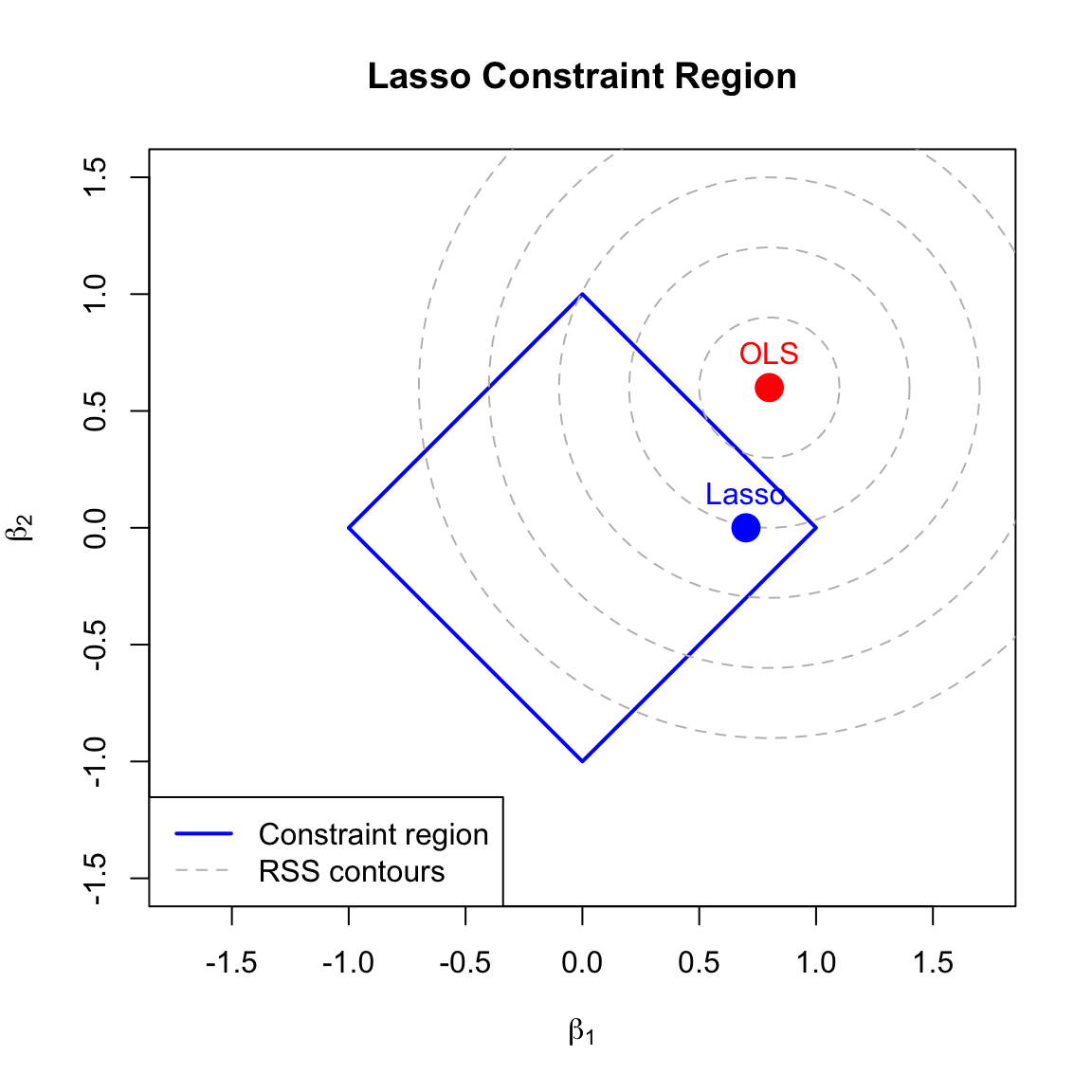
Lasso constrains coefficients to lie within a diamond (in 2D, an L1 ball):

\[\sum_{j=1}^p |\beta_j| \leq t\]

The diamond has corners on the axes, so the RSS contours often touch the constraint at a corner, forcing some coefficients to exactly zero.

Code

# Diamond constraint
diamond_x <- c(0, 1, 0, -1, 0)
diamond_y <- c(1, 0, -1, 0, 1)

plot(diamond_x, diamond_y, type = "l", lwd = 2, col = "blue",
     asp = 1, xlim = c(-1.5, 1.5), ylim = c(-1.5, 1.5),
     xlab = expression(beta[1]), ylab = expression(beta[2]),
     main = "Lasso Constraint Region")

# Add contours
for (r in seq(0.3, 1.5, 0.3)) {
  lines(r * cos(theta) + 0.8, r * sin(theta) + 0.6,
        col = "gray", lty = 2)
}

# OLS estimate
points(0.8, 0.6, pch = 19, cex = 2, col = "red")
text(0.8, 0.75, "OLS", col = "red")

# Lasso estimate (at corner)
points(0.7, 0, pch = 19, cex = 2, col = "blue")
text(0.7, 0.15, "Lasso", col = "blue")

legend("bottomleft", c("Constraint region", "RSS contours"),
       col = c("blue", "gray"), lty = c(1, 2), lwd = c(2, 1))

Figure 31.4: Geometric interpretation of lasso: the constraint region has corners on the axes, so the solution often lies at a corner where one or more coefficients are exactly zero

31.5 Elastic Net: Combining Ridge and Lasso

Elastic net combines both penalties:

\[P(\beta) = \alpha \sum_{j=1}^p |\beta_j| + (1-\alpha) \sum_{j=1}^p \beta_j^2\]

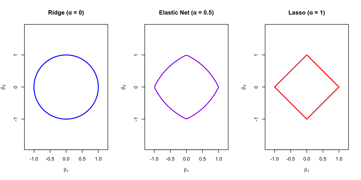
The mixing parameter $\alpha$ controls the balance between the two penalties. When $\alpha = 0$, elastic net reduces to pure ridge regression. When $\alpha = 1$, it becomes pure lasso. Values between 0 and 1 give a combination of both penalties, often with $\alpha = 0.5$ as a natural starting point.

Elastic net is often preferred when predictors are correlated. Unlike lasso, which arbitrarily selects one variable from a correlated group, elastic net tends to select groups of correlated variables together. This behavior often produces more stable and interpretable models when the underlying science suggests that correlated predictors genuinely contribute to the outcome.

Code

# Fit elastic net
enet_fit <- glmnet(X, y, alpha = 0.5)

plot(enet_fit, xvar = "lambda", main = "Elastic Net Coefficients (α = 0.5)")

Figure 31.5: Elastic net coefficient paths with alpha = 0.5 (equal mix of L1 and L2 penalties)

Code

par(mfrow = c(1, 3))

# Ridge
plot(cos(theta), sin(theta), type = "l", lwd = 2, col = "blue",
     asp = 1, xlim = c(-1.2, 1.2), ylim = c(-1.2, 1.2),
     xlab = expression(beta[1]), ylab = expression(beta[2]),
     main = "Ridge (α = 0)")

# Elastic net
alpha_en <- 0.5
en_x <- en_y <- numeric(100)
for (i in 1:100) {
  # Approximate elastic net constraint boundary
  ang <- theta[i]
  r <- 1 / (alpha_en * (abs(cos(ang)) + abs(sin(ang))) + (1 - alpha_en))
  en_x[i] <- r * cos(ang)
  en_y[i] <- r * sin(ang)
}
plot(en_x, en_y, type = "l", lwd = 2, col = "purple",
     asp = 1, xlim = c(-1.2, 1.2), ylim = c(-1.2, 1.2),
     xlab = expression(beta[1]), ylab = expression(beta[2]),
     main = "Elastic Net (α = 0.5)")

# Lasso
plot(diamond_x, diamond_y, type = "l", lwd = 2, col = "red",
     asp = 1, xlim = c(-1.2, 1.2), ylim = c(-1.2, 1.2),
     xlab = expression(beta[1]), ylab = expression(beta[2]),
     main = "Lasso (α = 1)")

Figure 31.6: Elastic net constraint region: intermediate between ridge (circle) and lasso (diamond)

31.6 Choosing Lambda with Cross-Validation

The regularization parameter $\lambda$ is typically chosen by cross-validation:

Code

# Cross-validation for lasso
set.seed(123)
cv_lasso <- cv.glmnet(X, y, alpha = 1)

# Plot cross-validation results
plot(cv_lasso)

# Optimal lambda values
cat("Lambda with minimum CV error:", round(cv_lasso$lambda.min, 4), "\n")

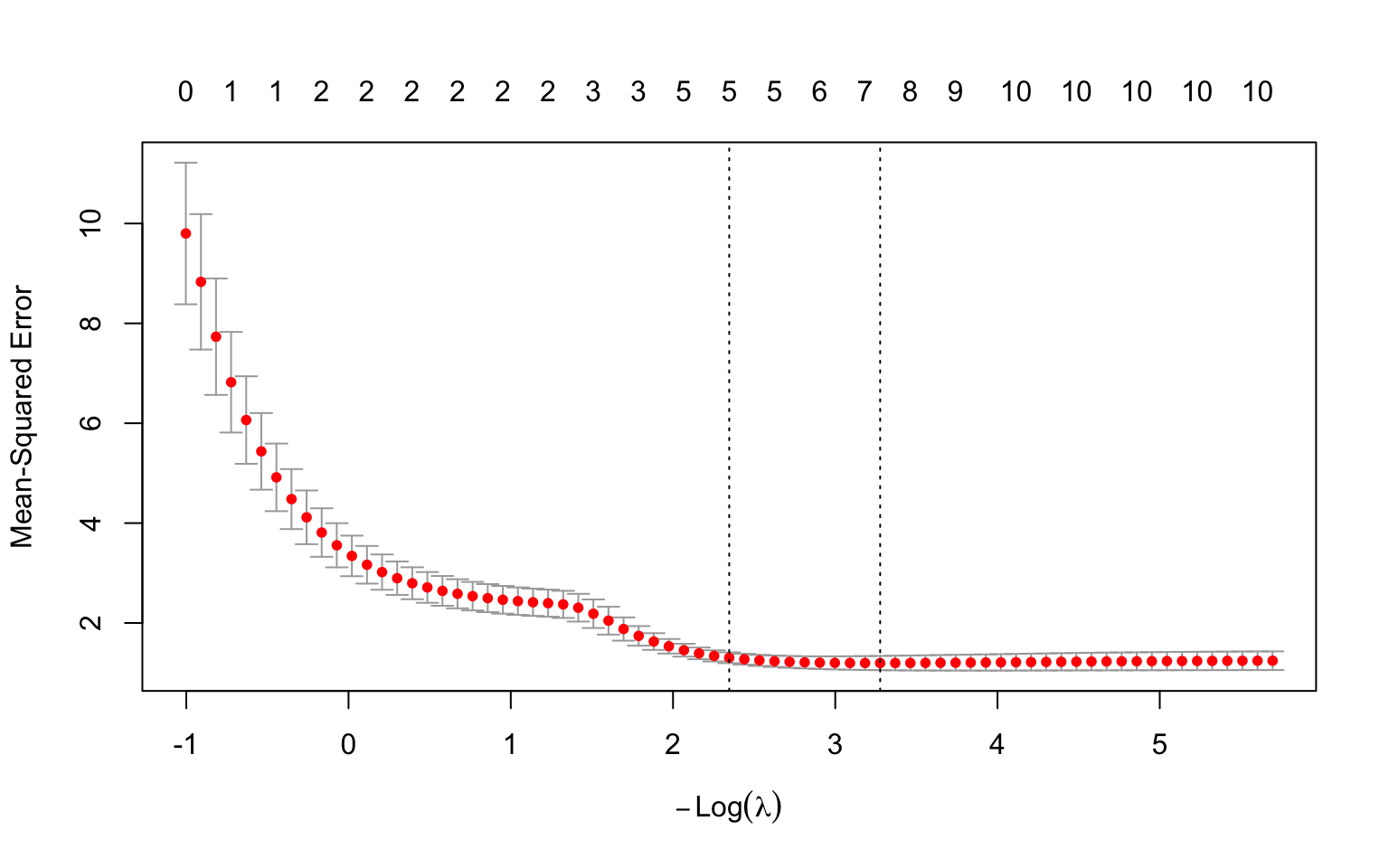
Lambda with minimum CV error: 0.0378

Code

cat("Lambda within 1 SE of minimum:", round(cv_lasso$lambda.1se, 4), "\n")

Lambda within 1 SE of minimum: 0.0957

Figure 31.7: Cross-validation to select optimal lambda: the left dashed line marks the minimum error, the right marks the most regularized model within one standard error

The lambda.1se (one standard error rule) often provides a more parsimonious model with nearly as good performance as the minimum.

Extracting Coefficients

Code

# Coefficients at different lambda values
cat("\nCoefficients at lambda.min:\n")


Coefficients at lambda.min:

Code

coef(cv_lasso, s = "lambda.min")

11 x 1 sparse Matrix of class "dgCMatrix"
              lambda.min
(Intercept)  0.095754403
V1           2.767360455
V2          -1.859381388
V3           1.597508497
V4          -0.099434052
V5           .          
V6           0.029276120
V7           .          
V8           .          
V9           0.005843271
V10         -0.082824940

Code

cat("\nCoefficients at lambda.1se:\n")


Coefficients at lambda.1se:

Code

coef(cv_lasso, s = "lambda.1se")

11 x 1 sparse Matrix of class "dgCMatrix"
             lambda.1se
(Intercept)  0.12555152
V1           2.16091712
V2          -1.35004269
V3           1.62087619
V4          -0.04486516
V5           .         
V6           .         
V7           .         
V8           .         
V9           .         
V10         -0.03937774

31.7 Comparing Regularization Methods

Let’s compare OLS, ridge, and lasso on the same data:

Code

# Fit models with optimal lambda
ridge_cv <- cv.glmnet(X, y, alpha = 0)
lasso_cv <- cv.glmnet(X, y, alpha = 1)

# Extract coefficients
coef_ols <- coef(lm(y ~ X))
coef_ridge <- coef(ridge_cv, s = "lambda.1se")
coef_lasso <- coef(lasso_cv, s = "lambda.1se")

# Compare (excluding intercept)
comparison <- data.frame(
  True = c(NA, true_beta),
  OLS = as.vector(coef_ols),
  Ridge = as.vector(coef_ridge),
  Lasso = as.vector(coef_lasso)
)
rownames(comparison) <- c("Intercept", paste0("X", 1:p))
round(comparison, 3)

          True    OLS  Ridge  Lasso
Intercept   NA  0.069  0.175  0.121
X1         3.0  3.214  1.587  2.248
X2        -2.0 -2.217 -0.764 -1.423
X3         1.5  1.559  1.499  1.618
X4         0.0 -0.126 -0.157 -0.053
X5         0.0 -0.061 -0.009  0.000
X6         0.0  0.103 -0.009  0.000
X7         0.0 -0.023 -0.008  0.000
X8         0.0  0.036  0.009  0.000
X9         0.0  0.051  0.081  0.000
X10        0.0 -0.113 -0.127 -0.046

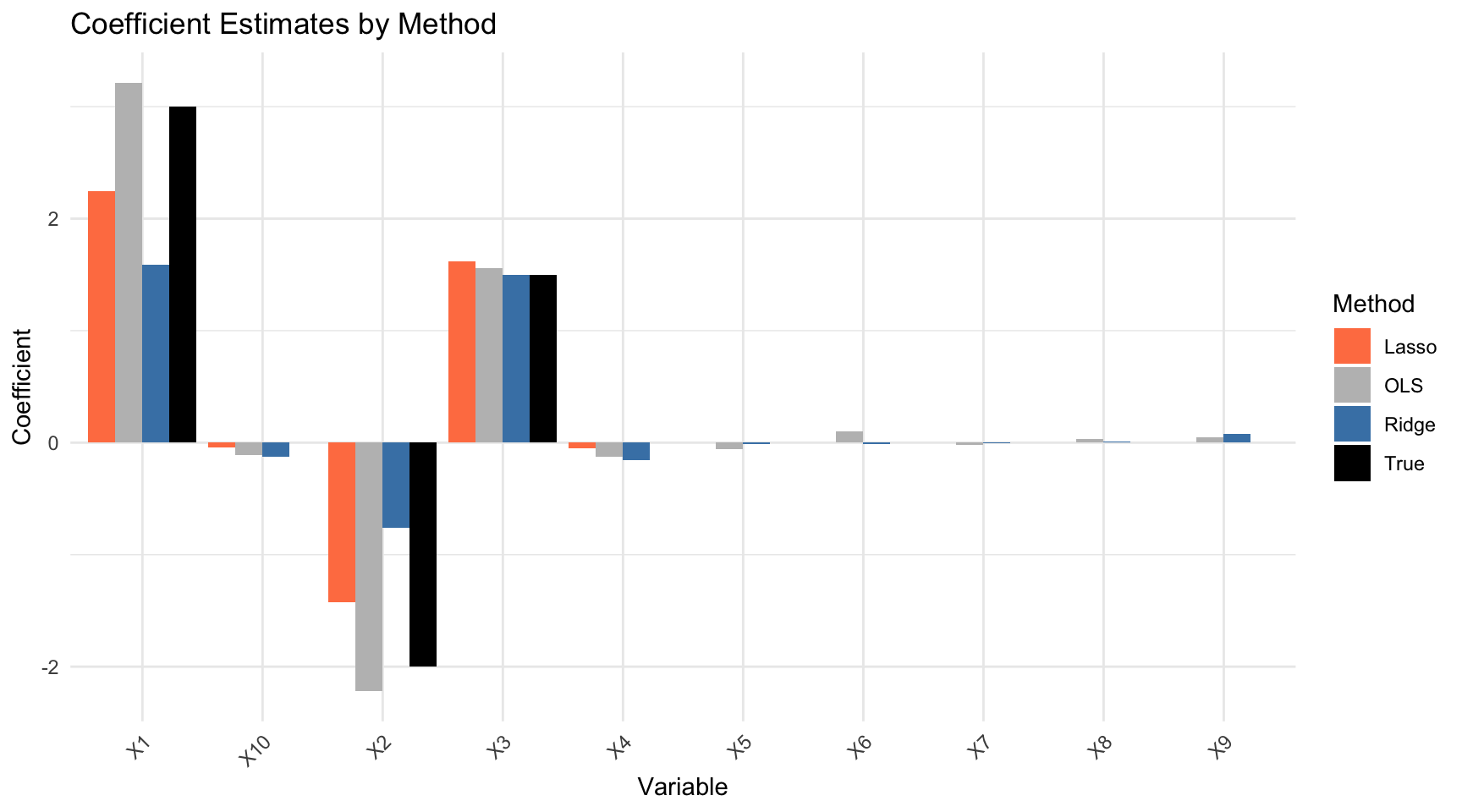
The comparison reveals the distinct behavior of each method. OLS estimates show high variance, especially for the variables whose true coefficients are zero—these spuriously appear nonzero due to fitting noise. Ridge shrinks all coefficients toward zero, reducing variance, but it doesn’t eliminate any predictors from the model. Lasso strikes a different balance: it correctly identifies many of the zero coefficients and sets them exactly to zero, producing a sparse model that more closely matches the true data-generating process.

31.8 Visualizing the Comparison

Code

# Plot comparison
var_names <- paste0("X", 1:p)
coef_df <- data.frame(
  Variable = rep(var_names, 4),
  Method = rep(c("True", "OLS", "Ridge", "Lasso"), each = p),
  Coefficient = c(true_beta,
                  as.vector(coef_ols)[-1],
                  as.vector(coef_ridge)[-1],
                  as.vector(coef_lasso)[-1])
)

ggplot(coef_df, aes(x = Variable, y = Coefficient, fill = Method)) +
  geom_bar(stat = "identity", position = "dodge") +
  scale_fill_manual(values = c("True" = "black", "OLS" = "gray",
                               "Ridge" = "steelblue", "Lasso" = "coral")) +
  theme(axis.text.x = element_text(angle = 45, hjust = 1)) +
  labs(title = "Coefficient Estimates by Method")

Figure 31.8: Comparison of coefficient estimates: true values, OLS, ridge, and lasso. Lasso successfully identifies zero coefficients while ridge shrinks but retains all.

31.9 Prediction Performance

Code

# Generate test data
set.seed(999)
X_test <- matrix(rnorm(50 * p), 50, p)
X_test[, 2] <- X_test[, 1] + rnorm(50, sd = 0.5)
X_test[, 3] <- X_test[, 1] + rnorm(50, sd = 0.5)
y_test <- X_test %*% true_beta + rnorm(50)

# Predictions
pred_ols <- predict(lm(y ~ X), newdata = data.frame(X_test))
pred_ridge <- predict(ridge_cv, newx = X_test, s = "lambda.1se")
pred_lasso <- predict(lasso_cv, newx = X_test, s = "lambda.1se")

# Test MSE
mse_ols <- mean((y_test - pred_ols)^2)

Error in `h()`:
! error in evaluating the argument 'x' in selecting a method for function 'mean': dims [product 50] do not match the length of object [100]

Code

mse_ridge <- mean((y_test - pred_ridge)^2)
mse_lasso <- mean((y_test - pred_lasso)^2)

cat("Test MSE:\n")

Test MSE:

Code

cat("  OLS:", round(mse_ols, 3), "\n")

Error:
! object 'mse_ols' not found

Code

cat("  Ridge:", round(mse_ridge, 3), "\n")

  Ridge: 1.642

Code

cat("  Lasso:", round(mse_lasso, 3), "\n")

  Lasso: 1.148

31.10 When to Use Each Method

Choosing among regularization methods depends on your goals and the structure of your data.

Ridge regression is the natural choice when you believe all predictors are genuinely relevant to the outcome, even if their individual effects are small. It is particularly effective when predictors are highly correlated, as the L2 penalty stabilizes coefficient estimates. Ridge tends to produce the most stable predictions, though the resulting model includes all variables, which may complicate interpretation.

Lasso is preferred when you want automatic variable selection and believe only a subset of predictors are truly relevant. The resulting sparse models are easier to interpret and communicate, since they explicitly identify which variables matter. However, lasso can behave arbitrarily when predictors are correlated, selecting one while zeroing out others that may be equally important.

Elastic net offers a middle ground that is often optimal in practice. Use it when predictors are correlated but you still want variable selection—elastic net tends to select groups of correlated variables together rather than making arbitrary choices. It’s also a sensible default when you’re unsure whether ridge or lasso is more appropriate, as cross-validation can select an optimal mixing parameter.

One practical note: always standardize predictors before applying regularization, as the penalty treats all coefficients equally and would otherwise penalize variables on larger scales more heavily. The glmnet function handles this automatically by default.

31.11 Regularization in Practice

High-Dimensional Data Example

Regularization is especially valuable when $p$ approaches or exceeds $n$:

Code

# High-dimensional example: p = 80, n = 100
set.seed(42)
n <- 100
p <- 80
X_hd <- matrix(rnorm(n * p), n, p)
# Sparse true model: only 5 predictors matter
true_beta_hd <- c(rep(2, 5), rep(0, p - 5))
y_hd <- X_hd %*% true_beta_hd + rnorm(n)

# OLS fails (numerically unstable or overfits severely)
# ols_hd <- lm(y_hd ~ X_hd)  # Would have issues

# Lasso works
cv_lasso_hd <- cv.glmnet(X_hd, y_hd, alpha = 1)

# How many non-zero coefficients?
lasso_coef <- coef(cv_lasso_hd, s = "lambda.1se")
n_nonzero <- sum(lasso_coef[-1] != 0)
cat("True non-zero coefficients:", 5, "\n")

True non-zero coefficients: 5

Code

cat("Lasso selected:", n_nonzero, "\n")

Lasso selected: 5

Code

# Which variables selected?
selected <- which(lasso_coef[-1] != 0)
cat("Selected variables:", paste(selected, collapse = ", "), "\n")

Selected variables: 1, 2, 3, 4, 5

Regularized Logistic Regression

Regularization extends naturally to classification problems:

Code

# Binary classification example
set.seed(42)
y_binary <- rbinom(n, 1, plogis(X %*% c(1, -0.5, 0.3, rep(0, p - 3))))

Error in `X %*% c(1, -0.5, 0.3, rep(0, p - 3))`:
! non-conformable arguments

Code

# Regularized logistic regression
cv_logit <- cv.glmnet(X, y_binary, family = "binomial", alpha = 1)

Error in `h()`:
! error in evaluating the argument 'x' in selecting a method for function 'drop': object 'y_binary' not found

Code

# Coefficients
cat("Selected predictors for logistic regression:\n")

Selected predictors for logistic regression:

Code

logit_coef <- coef(cv_logit, s = "lambda.1se")

Error:
! object 'cv_logit' not found

Code

which(logit_coef[-1] != 0)

Error in `h()`:
! error in evaluating the argument 'x' in selecting a method for function 'which': object 'logit_coef' not found

31.12 Exercises

Exercise Reg.1: Ridge vs Lasso

Generate data with $n = 100$ observations and $p = 20$ predictors where:
- Predictors 1-3 have coefficients 3, -2, 1
- Predictors 4-6 are correlated with 1-3
- Predictors 7-20 have coefficient 0
Fit OLS, ridge, and lasso. Compare the coefficient estimates to the true values.
Generate a test set and compare prediction performance.

Exercise Reg.2: Choosing Alpha

For the data above, use cross-validation to select the optimal mixing parameter $\alpha$ for elastic net. Try $\alpha \in \{0, 0.25, 0.5, 0.75, 1\}$.
Does the optimal $\alpha$ match what you would expect given the correlation structure?

Exercise Reg.3: High-Dimensional Classification

Load a gene expression dataset with many more genes than samples. Use regularized logistic regression to build a classifier.
Compare the number of genes selected by lasso at lambda.min vs lambda.1se. Which would you prefer in practice?

31.13 Summary

This chapter introduced regularization as a powerful technique for preventing overfitting, especially when the number of predictors is large relative to the sample size. The core idea is to add a penalty term that shrinks coefficients toward zero, trading a small increase in bias for a substantial reduction in variance.

Ridge regression uses an L2 penalty (sum of squared coefficients) that shrinks all coefficients toward zero but never exactly to zero. This makes ridge ideal when all predictors may be relevant and particularly effective for handling multicollinearity. Lasso regression uses an L1 penalty (sum of absolute values) that can shrink coefficients exactly to zero, automatically performing variable selection. The resulting sparse models are easier to interpret, though lasso can behave arbitrarily with correlated predictors. Elastic net combines both penalties, offering the variable selection of lasso with the stability of ridge for correlated predictors.

The regularization parameter $\lambda$ controls the penalty strength and is typically selected by cross-validation. The lambda.min value minimizes cross-validation error, while the lambda.1se (one standard error rule) often provides a more parsimonious model with nearly equivalent performance.

Standardization of predictors is essential before applying regularization, since the penalty treats all coefficients equally and would otherwise unfairly penalize variables measured on larger scales. Finally, regularization extends naturally beyond regression to classification problems through regularized logistic regression and other generalized linear models.

31.14 Additional Resources

James et al. (2023) - Detailed treatment of regularization methods
Hastie, Tibshirani, and Friedman (2009) - Theoretical foundations
glmnet package vignette - Practical implementation details
Tibshirani (1996) - Original lasso paper

# Regularization Methods {#sec-regularization} ```{r} #| echo: false #| message: false library(tidyverse) library(glmnet) theme_set(theme_minimal()) ``` ## The Need for Regularization Standard linear regression estimates coefficients by minimizing the residual sum of squares (RSS): $$\text{RSS} = \sum_{i=1}^n \left(y_i - \beta_0 - \sum_{j=1}^p \beta_j x_{ij}\right)^2$$ This works well when you have many more observations than predictors ($n \gg p$) and the predictors are not highly correlated. But problems arise in several common situations. When you have **many predictors** relative to the number of observations, coefficient estimates become unstable and their variance is high. The model has too many degrees of freedom to estimate reliably from the available data. When predictors are **highly correlated** (multicollinearity), the problem is compounded: small changes in the data can cause dramatic swings in the estimated coefficients, even though predictions remain stable. In either case, the result is often **overfitting**—the model fits the training data well but predicts poorly on new observations. **Regularization** addresses these issues by adding a penalty term that shrinks coefficients toward zero. This intentionally introduces a small amount of bias in exchange for a substantial reduction in variance. The net effect is usually better predictions on new data, especially when the number of predictors is large relative to the sample size. ## The Regularization Idea Regularized regression minimizes a modified objective: $$\text{Minimize: } \text{RSS} + \lambda \cdot P(\beta)$$ In this formulation, $P(\beta)$ is a **penalty function** that penalizes large coefficients, and $\lambda \geq 0$ is the **regularization parameter** that controls the strength of the penalty. The effect of the penalty is to shrink coefficients toward zero, with $\lambda$ controlling how aggressively. When $\lambda = 0$, there is no penalty and we recover ordinary least squares. As $\lambda$ increases, the penalty becomes stronger and coefficients shrink more. In the limit as $\lambda \to \infty$, all coefficients are forced to zero. Different choices of the penalty function $P(\beta)$ lead to different regularization methods, each with distinct properties and use cases. ## Ridge Regression (L2 Penalty) **Ridge regression** [@hoerl1970ridge] uses the sum of squared coefficients as the penalty: $$P(\beta) = \sum_{j=1}^p \beta_j^2$$ The full optimization problem is: $$\hat{\beta}^{\text{ridge}} = \arg\min_\beta \left\{ \sum_{i=1}^n \left(y_i - \beta_0 - \sum_{j=1}^p \beta_j x_{ij}\right)^2 + \lambda \sum_{j=1}^p \beta_j^2 \right\}$$ ### Properties of Ridge Regression Ridge regression shrinks all coefficients toward zero but **never exactly to zero**. This means all predictors remain in the model regardless of how large $\lambda$ becomes—coefficients get very small but never vanish entirely. This property makes ridge regression particularly useful when you believe all predictors are relevant to some degree. It is also especially effective when predictors are highly correlated (multicollinearity), as the penalty stabilizes the coefficient estimates that would otherwise be wildly unstable in ordinary least squares. ```{r} #| label: fig-ridge-path #| fig-cap: "Ridge regression coefficient paths: as lambda increases, coefficients shrink toward zero but never reach exactly zero" #| fig-width: 8 #| fig-height: 5 # Generate sample data with correlated predictors set.seed(42) n <- 100 p <- 10 X <- matrix(rnorm(n * p), n, p) # Create correlated predictors X[, 2] <- X[, 1] + rnorm(n, sd = 0.5) X[, 3] <- X[, 1] + rnorm(n, sd = 0.5) true_beta <- c(3, -2, 1.5, rep(0, p - 3)) y <- X %*% true_beta + rnorm(n) # Fit ridge regression across lambda values ridge_fit <- glmnet(X, y, alpha = 0) # alpha = 0 for ridge # Plot coefficient paths plot(ridge_fit, xvar = "lambda", main = "Ridge Regression Coefficients") ``` ### Geometric Interpretation Ridge regression constrains coefficients to lie within a sphere (in 2D, a circle) centered at the origin: $$\sum_{j=1}^p \beta_j^2 \leq t$$ where $t$ is inversely related to $\lambda$. The OLS solution may lie outside this constraint region, so ridge finds the point where the RSS contours first touch the constraint boundary. ```{r} #| label: fig-ridge-geometry #| fig-cap: "Geometric interpretation of ridge regression: the constraint region is circular, so the solution rarely lies exactly on an axis (coefficient rarely zero)" #| fig-width: 6 #| fig-height: 6 # Geometric illustration theta <- seq(0, 2*pi, length.out = 100) plot(cos(theta), sin(theta), type = "l", lwd = 2, col = "blue", asp = 1, xlim = c(-1.5, 1.5), ylim = c(-1.5, 1.5), xlab = expression(beta[1]), ylab = expression(beta[2]), main = "Ridge Constraint Region") # Add contours representing RSS for (r in seq(0.3, 1.5, 0.3)) { lines(r * cos(theta) + 0.8, r * sin(theta) + 0.6, col = "gray", lty = 2) } # OLS estimate points(0.8, 0.6, pch = 19, cex = 2, col = "red") text(0.8, 0.75, "OLS", col = "red") # Ridge estimate (on boundary) points(0.5, 0.37, pch = 19, cex = 2, col = "blue") text(0.5, 0.5, "Ridge", col = "blue") legend("bottomleft", c("Constraint region", "RSS contours"), col = c("blue", "gray"), lty = c(1, 2), lwd = c(2, 1)) ``` ## Lasso Regression (L1 Penalty) **Lasso** (Least Absolute Shrinkage and Selection Operator) [@tibshirani1996regression] uses the sum of absolute values as the penalty: $$P(\beta) = \sum_{j=1}^p |\beta_j|$$ The optimization problem is: $$\hat{\beta}^{\text{lasso}} = \arg\min_\beta \left\{ \sum_{i=1}^n \left(y_i - \beta_0 - \sum_{j=1}^p \beta_j x_{ij}\right)^2 + \lambda \sum_{j=1}^p |\beta_j| \right\}$$ ### Properties of Lasso Regression Unlike ridge, lasso can shrink coefficients **exactly to zero**, effectively performing **variable selection**. This produces **sparse models** with fewer predictors, making the resulting models easier to interpret since they explicitly identify which variables are "important." However, lasso may struggle when predictors are highly correlated—in such cases, it tends to select one predictor from a correlated group arbitrarily while setting the others to zero, rather than distributing the effect among them as ridge would. ```{r} #| label: fig-lasso-path #| fig-cap: "Lasso regression coefficient paths: as lambda increases, coefficients shrink and some become exactly zero (variable selection)" #| fig-width: 8 #| fig-height: 5 # Fit lasso regression lasso_fit <- glmnet(X, y, alpha = 1) # alpha = 1 for lasso plot(lasso_fit, xvar = "lambda", main = "Lasso Regression Coefficients") ``` ### Geometric Interpretation Lasso constrains coefficients to lie within a diamond (in 2D, an L1 ball): $$\sum_{j=1}^p |\beta_j| \leq t$$ The diamond has corners on the axes, so the RSS contours often touch the constraint at a corner, forcing some coefficients to exactly zero. ```{r} #| label: fig-lasso-geometry #| fig-cap: "Geometric interpretation of lasso: the constraint region has corners on the axes, so the solution often lies at a corner where one or more coefficients are exactly zero" #| fig-width: 6 #| fig-height: 6 # Diamond constraint diamond_x <- c(0, 1, 0, -1, 0) diamond_y <- c(1, 0, -1, 0, 1) plot(diamond_x, diamond_y, type = "l", lwd = 2, col = "blue", asp = 1, xlim = c(-1.5, 1.5), ylim = c(-1.5, 1.5), xlab = expression(beta[1]), ylab = expression(beta[2]), main = "Lasso Constraint Region") # Add contours for (r in seq(0.3, 1.5, 0.3)) { lines(r * cos(theta) + 0.8, r * sin(theta) + 0.6, col = "gray", lty = 2) } # OLS estimate points(0.8, 0.6, pch = 19, cex = 2, col = "red") text(0.8, 0.75, "OLS", col = "red") # Lasso estimate (at corner) points(0.7, 0, pch = 19, cex = 2, col = "blue") text(0.7, 0.15, "Lasso", col = "blue") legend("bottomleft", c("Constraint region", "RSS contours"), col = c("blue", "gray"), lty = c(1, 2), lwd = c(2, 1)) ``` ## Elastic Net: Combining Ridge and Lasso **Elastic net** combines both penalties: $$P(\beta) = \alpha \sum_{j=1}^p |\beta_j| + (1-\alpha) \sum_{j=1}^p \beta_j^2$$ The mixing parameter $\alpha$ controls the balance between the two penalties. When $\alpha = 0$, elastic net reduces to pure ridge regression. When $\alpha = 1$, it becomes pure lasso. Values between 0 and 1 give a combination of both penalties, often with $\alpha = 0.5$ as a natural starting point. Elastic net is often preferred when predictors are correlated. Unlike lasso, which arbitrarily selects one variable from a correlated group, elastic net tends to select groups of correlated variables together. This behavior often produces more stable and interpretable models when the underlying science suggests that correlated predictors genuinely contribute to the outcome. ```{r} #| label: fig-elastic-net #| fig-cap: "Elastic net coefficient paths with alpha = 0.5 (equal mix of L1 and L2 penalties)" #| fig-width: 8 #| fig-height: 5 # Fit elastic net enet_fit <- glmnet(X, y, alpha = 0.5) plot(enet_fit, xvar = "lambda", main = "Elastic Net Coefficients (α = 0.5)") ``` ```{r} #| label: fig-enet-geometry #| fig-cap: "Elastic net constraint region: intermediate between ridge (circle) and lasso (diamond)" #| fig-width: 8 #| fig-height: 4 par(mfrow = c(1, 3)) # Ridge plot(cos(theta), sin(theta), type = "l", lwd = 2, col = "blue", asp = 1, xlim = c(-1.2, 1.2), ylim = c(-1.2, 1.2), xlab = expression(beta[1]), ylab = expression(beta[2]), main = "Ridge (α = 0)") # Elastic net alpha_en <- 0.5 en_x <- en_y <- numeric(100) for (i in 1:100) { # Approximate elastic net constraint boundary ang <- theta[i] r <- 1 / (alpha_en * (abs(cos(ang)) + abs(sin(ang))) + (1 - alpha_en)) en_x[i] <- r * cos(ang) en_y[i] <- r * sin(ang) } plot(en_x, en_y, type = "l", lwd = 2, col = "purple", asp = 1, xlim = c(-1.2, 1.2), ylim = c(-1.2, 1.2), xlab = expression(beta[1]), ylab = expression(beta[2]), main = "Elastic Net (α = 0.5)") # Lasso plot(diamond_x, diamond_y, type = "l", lwd = 2, col = "red", asp = 1, xlim = c(-1.2, 1.2), ylim = c(-1.2, 1.2), xlab = expression(beta[1]), ylab = expression(beta[2]), main = "Lasso (α = 1)") ``` ## Choosing Lambda with Cross-Validation The regularization parameter $\lambda$ is typically chosen by cross-validation: ```{r} #| label: fig-cv-lambda #| fig-cap: "Cross-validation to select optimal lambda: the left dashed line marks the minimum error, the right marks the most regularized model within one standard error" #| fig-width: 8 #| fig-height: 5 # Cross-validation for lasso set.seed(123) cv_lasso <- cv.glmnet(X, y, alpha = 1) # Plot cross-validation results plot(cv_lasso) # Optimal lambda values cat("Lambda with minimum CV error:", round(cv_lasso$lambda.min, 4), "\n") cat("Lambda within 1 SE of minimum:", round(cv_lasso$lambda.1se, 4), "\n") ``` The `lambda.1se` (one standard error rule) often provides a more parsimonious model with nearly as good performance as the minimum. ### Extracting Coefficients ```{r} # Coefficients at different lambda values cat("\nCoefficients at lambda.min:\n") coef(cv_lasso, s = "lambda.min") cat("\nCoefficients at lambda.1se:\n") coef(cv_lasso, s = "lambda.1se") ``` ## Comparing Regularization Methods Let's compare OLS, ridge, and lasso on the same data: ```{r} # Fit models with optimal lambda ridge_cv <- cv.glmnet(X, y, alpha = 0) lasso_cv <- cv.glmnet(X, y, alpha = 1) # Extract coefficients coef_ols <- coef(lm(y ~ X)) coef_ridge <- coef(ridge_cv, s = "lambda.1se") coef_lasso <- coef(lasso_cv, s = "lambda.1se") # Compare (excluding intercept) comparison <- data.frame( True = c(NA, true_beta), OLS = as.vector(coef_ols), Ridge = as.vector(coef_ridge), Lasso = as.vector(coef_lasso) ) rownames(comparison) <- c("Intercept", paste0("X", 1:p)) round(comparison, 3) ``` The comparison reveals the distinct behavior of each method. **OLS** estimates show high variance, especially for the variables whose true coefficients are zero—these spuriously appear nonzero due to fitting noise. **Ridge** shrinks all coefficients toward zero, reducing variance, but it doesn't eliminate any predictors from the model. **Lasso** strikes a different balance: it correctly identifies many of the zero coefficients and sets them exactly to zero, producing a sparse model that more closely matches the true data-generating process. ## Visualizing the Comparison ```{r} #| label: fig-method-comparison #| fig-cap: "Comparison of coefficient estimates: true values, OLS, ridge, and lasso. Lasso successfully identifies zero coefficients while ridge shrinks but retains all." #| fig-width: 9 #| fig-height: 5 # Plot comparison var_names <- paste0("X", 1:p) coef_df <- data.frame( Variable = rep(var_names, 4), Method = rep(c("True", "OLS", "Ridge", "Lasso"), each = p), Coefficient = c(true_beta, as.vector(coef_ols)[-1], as.vector(coef_ridge)[-1], as.vector(coef_lasso)[-1]) ) ggplot(coef_df, aes(x = Variable, y = Coefficient, fill = Method)) + geom_bar(stat = "identity", position = "dodge") + scale_fill_manual(values = c("True" = "black", "OLS" = "gray", "Ridge" = "steelblue", "Lasso" = "coral")) + theme(axis.text.x = element_text(angle = 45, hjust = 1)) + labs(title = "Coefficient Estimates by Method") ``` ## Prediction Performance ```{r} # Generate test data set.seed(999) X_test <- matrix(rnorm(50 * p), 50, p) X_test[, 2] <- X_test[, 1] + rnorm(50, sd = 0.5) X_test[, 3] <- X_test[, 1] + rnorm(50, sd = 0.5) y_test <- X_test %*% true_beta + rnorm(50) # Predictions pred_ols <- predict(lm(y ~ X), newdata = data.frame(X_test)) pred_ridge <- predict(ridge_cv, newx = X_test, s = "lambda.1se") pred_lasso <- predict(lasso_cv, newx = X_test, s = "lambda.1se") # Test MSE mse_ols <- mean((y_test - pred_ols)^2) mse_ridge <- mean((y_test - pred_ridge)^2) mse_lasso <- mean((y_test - pred_lasso)^2) cat("Test MSE:\n") cat(" OLS:", round(mse_ols, 3), "\n") cat(" Ridge:", round(mse_ridge, 3), "\n") cat(" Lasso:", round(mse_lasso, 3), "\n") ``` ## When to Use Each Method Choosing among regularization methods depends on your goals and the structure of your data. **Ridge regression** is the natural choice when you believe all predictors are genuinely relevant to the outcome, even if their individual effects are small. It is particularly effective when predictors are highly correlated, as the L2 penalty stabilizes coefficient estimates. Ridge tends to produce the most stable predictions, though the resulting model includes all variables, which may complicate interpretation. **Lasso** is preferred when you want automatic variable selection and believe only a subset of predictors are truly relevant. The resulting sparse models are easier to interpret and communicate, since they explicitly identify which variables matter. However, lasso can behave arbitrarily when predictors are correlated, selecting one while zeroing out others that may be equally important. **Elastic net** offers a middle ground that is often optimal in practice. Use it when predictors are correlated but you still want variable selection—elastic net tends to select groups of correlated variables together rather than making arbitrary choices. It's also a sensible default when you're unsure whether ridge or lasso is more appropriate, as cross-validation can select an optimal mixing parameter. One practical note: always standardize predictors before applying regularization, as the penalty treats all coefficients equally and would otherwise penalize variables on larger scales more heavily. The `glmnet` function handles this automatically by default. ## Regularization in Practice ### High-Dimensional Data Example Regularization is especially valuable when $p$ approaches or exceeds $n$: ```{r} #| label: fig-high-dim #| fig-cap: "Regularization is essential for high-dimensional data where p ≈ n or p > n" #| fig-width: 8 #| fig-height: 5 # High-dimensional example: p = 80, n = 100 set.seed(42) n <- 100 p <- 80 X_hd <- matrix(rnorm(n * p), n, p) # Sparse true model: only 5 predictors matter true_beta_hd <- c(rep(2, 5), rep(0, p - 5)) y_hd <- X_hd %*% true_beta_hd + rnorm(n) # OLS fails (numerically unstable or overfits severely) # ols_hd <- lm(y_hd ~ X_hd) # Would have issues # Lasso works cv_lasso_hd <- cv.glmnet(X_hd, y_hd, alpha = 1) # How many non-zero coefficients? lasso_coef <- coef(cv_lasso_hd, s = "lambda.1se") n_nonzero <- sum(lasso_coef[-1] != 0) cat("True non-zero coefficients:", 5, "\n") cat("Lasso selected:", n_nonzero, "\n") # Which variables selected? selected <- which(lasso_coef[-1] != 0) cat("Selected variables:", paste(selected, collapse = ", "), "\n") ``` ### Regularized Logistic Regression Regularization extends naturally to classification problems: ```{r} # Binary classification example set.seed(42) y_binary <- rbinom(n, 1, plogis(X %*% c(1, -0.5, 0.3, rep(0, p - 3)))) # Regularized logistic regression cv_logit <- cv.glmnet(X, y_binary, family = "binomial", alpha = 1) # Coefficients cat("Selected predictors for logistic regression:\n") logit_coef <- coef(cv_logit, s = "lambda.1se") which(logit_coef[-1] != 0) ``` ## Exercises ::: {.callout-note} ### Exercise Reg.1: Ridge vs Lasso 1. Generate data with $n = 100$ observations and $p = 20$ predictors where: - Predictors 1-3 have coefficients 3, -2, 1 - Predictors 4-6 are correlated with 1-3 - Predictors 7-20 have coefficient 0 2. Fit OLS, ridge, and lasso. Compare the coefficient estimates to the true values. 3. Generate a test set and compare prediction performance. ::: ::: {.callout-note} ### Exercise Reg.2: Choosing Alpha 4. For the data above, use cross-validation to select the optimal mixing parameter $\alpha$ for elastic net. Try $\alpha \in \{0, 0.25, 0.5, 0.75, 1\}$. 5. Does the optimal $\alpha$ match what you would expect given the correlation structure? ::: ::: {.callout-note} ### Exercise Reg.3: High-Dimensional Classification 6. Load a gene expression dataset with many more genes than samples. Use regularized logistic regression to build a classifier. 7. Compare the number of genes selected by lasso at `lambda.min` vs `lambda.1se`. Which would you prefer in practice? ::: ## Summary This chapter introduced **regularization** as a powerful technique for preventing overfitting, especially when the number of predictors is large relative to the sample size. The core idea is to add a penalty term that shrinks coefficients toward zero, trading a small increase in bias for a substantial reduction in variance. **Ridge regression** uses an L2 penalty (sum of squared coefficients) that shrinks all coefficients toward zero but never exactly to zero. This makes ridge ideal when all predictors may be relevant and particularly effective for handling multicollinearity. **Lasso regression** uses an L1 penalty (sum of absolute values) that can shrink coefficients exactly to zero, automatically performing variable selection. The resulting sparse models are easier to interpret, though lasso can behave arbitrarily with correlated predictors. **Elastic net** combines both penalties, offering the variable selection of lasso with the stability of ridge for correlated predictors. The regularization parameter $\lambda$ controls the penalty strength and is typically selected by **cross-validation**. The `lambda.min` value minimizes cross-validation error, while the `lambda.1se` (one standard error rule) often provides a more parsimonious model with nearly equivalent performance. **Standardization** of predictors is essential before applying regularization, since the penalty treats all coefficients equally and would otherwise unfairly penalize variables measured on larger scales. Finally, regularization extends naturally beyond regression to classification problems through regularized logistic regression and other generalized linear models. ## Additional Resources - @james2023islr - Detailed treatment of regularization methods - @hastie2009elements - Theoretical foundations - `glmnet` package vignette - Practical implementation details - @tibshirani1996regression - Original lasso paper