Appendix C — Common Data Formats & Public Repositories
This appendix is a field guide to the file formats you will meet most often as a bioengineer working with data, and to the public repositories where published datasets, sequences, genomes, and structures live. It is meant to be scanned in about 15 minutes and returned to whenever you open an unfamiliar file or need to find a published dataset.
Why an appendix and not a tutorial? Recognizing file formats and navigating data repositories is a skill more than a procedure: every repository’s interface evolves, and the right portal depends on your question. The command-line tools used here (head, zcat, grep, wc, wget) are introduced in Chapter 5 and Lectures 03-05; see Chapter 9 for more grep. Terms are defined in the Glossary (Appendix J).
D Part 1 - Common file formats
A useful first question for any file: is it plain text or binary? Plain-text files can be inspected with head, less, and grep, versioned with Git, and read by any language decades from now. Binary files are smaller and faster but need specific software to open.
D.1 Plain-text tables: CSV and TSV
The workhorse of scientific data exchange. Each line is a row; columns are separated by commas (CSV, .csv) or tab characters (TSV, .tsv or .txt).
sample_id,material,stiffness_kPa,temp_C
S01,PEG_hydrogel,12.4,37
S02,PEG_hydrogel,13.1,37
S03,alginate,8.7,37- The first line is usually a header with column names.
- Follow tidy data conventions (Lecture 02): one variable per column, one observation per row, one value per cell.
- TSV is safer when text fields might contain commas (e.g., gene descriptions).
- Read in R with
readr::read_csv()/read_tsv(); in Python withpandas.read_csv()(addsep="\t"for TSV). - Quick shell checks:
head file.csv,wc -l file.csv(rows + header),cut -d, -f3 file.csv | sort | uniq -c(tabulate column 3).
D.2 Spreadsheets: Excel (.xlsx) and its caveats
Excel is fine for viewing and data entry, but it is risky as the only copy of your data:
- Automatic conversion: Excel silently converts some values. Gene symbols such as SEPT2, MARCH1, and DEC1 have been turned into dates (“2-Sep”, “1-Mar”), and long numeric IDs are converted to scientific notation, losing digits. A 2016 survey found these errors in roughly one-fifth of papers with supplementary Excel gene lists (Ziemann et al., 2016); HGNC later renamed several genes partly because of this (Bruford et al., 2020). Keeping raw data in plain text and doing all manipulation in code is one of the core recommendations of “good enough” scientific computing practice (Wilson et al., 2017).
- Hidden structure: merged cells, colors used as data, multiple tables per sheet, and formulas make files hard to read programmatically.
- Proprietary binary format:
.xlsxis a zipped XML bundle, so Git cannot show meaningful diffs.
Keep a CSV copy. Treat raw data as read-only, store a plain-text CSV (one sheet = one CSV) alongside any .xlsx, and do analysis in code. If you must import into Excel, use Data → From Text/CSV and set gene-name or ID columns to Text. In R, readxl::read_excel() reads .xlsx directly without Excel.
D.3 Sequences: FASTA
Plain text for DNA, RNA, or protein sequences. Each record is a header line starting with > followed by one or more lines of sequence:
>NM_000546.6 Homo sapiens tumor protein p53 (TP53), mRNA
CTCAAAAGTCTAGAGCCACCGTCCAGGGAGCAGGTAGCTGCTGGGCTCCGGGGACACTTTGCGTTCGGGC
TGGGAGCGTGCTTTCCACGACGGTGACACGCTTCCCTGGATTGGCAGCCAGACTGCCTTCCGGGTCACTG
>sp|P04637|P53_HUMAN Cellular tumor antigen p53
MEEPQSDPSVEPPLSQETFSDLWKLLPENNVLSPLPSQAMDDLMLSPDDIEQWFTEDPGP- Extensions:
.fa,.fasta,.fna(nucleotide),.faa(amino acid), often gzipped (.fa.gz). - Used for reference genomes, transcripts, primers, and protein sequences.
- No quality scores (contrast with FASTQ).
- Count records:
grep -c '>' file.fasta. List headers:grep '>' file.fasta | head.
D.4 Raw sequencing reads: FASTQ
Plain text with a strict 4-line-per-read structure (Table D.1):
@SRR12345.1 NS500126:1:H7TG3BGXY:1:11101:18923:1057
NCATGCAGCGTACGGTAATTGGCAGGCATTAGCAGCATCC
+
#AAAAFFFFFFFFFFFFFFFFFFFFFFFFFFFFFFFFFFF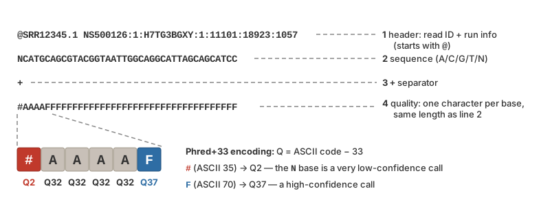
| Line | Content |
|---|---|
| 1 | Header: read ID plus instrument, run, lane, tile, and x/y position. Starts with @ |
| 2 | The sequence (A/C/G/T/N) |
| 3 | A + separator (sometimes repeats the header) |
| 4 | Per-base quality scores, one ASCII character per base, same length as line 2 |
Each quality character encodes a Phred score \(Q = -10 \log_{10}(P)\), where \(P\) is the probability that the base call is wrong (Table D.2):
| Phred Q | Error probability | Base-call accuracy |
|---|---|---|
| 10 | 1 in 10 | 90% |
| 20 | 1 in 100 | 99% |
| 30 | 1 in 1,000 | 99.9% |
| 40 | 1 in 10,000 | 99.99% |
Modern Illumina data use Phred+33 encoding: the character’s ASCII code minus 33 gives Q. So ! (ASCII 33) is Q0, + (43) is Q10, 5 (53) is Q20, ? (63) is Q30, and I (73) is Q40. In the example above, the leading # (Q2) on the N base signals a very low-confidence call.
- Paired-end runs produce two files per sample, typically
..._R1_001.fastq.gzand..._R2_001.fastq.gz; the reads in each file are in the same order. - Because each read is exactly 4 lines, number of reads = lines / 4:
echo $(( $(zcat reads.fastq.gz | wc -l) / 4 )). - Quality-control tools such as FastQC summarize quality scores across a whole file.
grep -c '^@'
It is tempting to count reads by counting header lines, since every header starts with @. But @ is also a valid quality character—ASCII 64, which in Phred+33 encodes Q31—so line 4 of a record can begin with @ too, and the count comes out too high. The structure of the file, not its characters, is what is reliable: count reads as lines divided by 4 (as above, or zcat reads.fastq.gz | awk 'NR % 4 == 1' | wc -l), and pull out sequences by line position (awk 'NR % 4 == 2') rather than by pattern matching.
D.5 Compressed files (.gz) and streaming
Sequencing and other large text files are almost always stored gzip-compressed (.gz), often 3-5x smaller. You rarely need to decompress them to disk; instead stream them through a pipe:
zcat reads.fastq.gz | head -n 8          # first two reads
zcat reads.fastq.gz | wc -l              # total lines
zcat genome.fa.gz | grep -c '>'          # number of sequences
zless annotation.gtf.gz                  # page through interactively

gzip results.tsv                         # compress (creates results.tsv.gz, removes original)
gunzip results.tsv.gz                    # decompress
gzip -k results.tsv                      # -k keeps the original
On macOS, the built-in zcat expects .Z files; use gzcat file.gz or zcat < file.gz instead. Some genomics files use bgzip (block gzip), which is still readable with zcat but also allows indexed random access (e.g., with tabix or samtools). Other archive types you will see: .zip (unzip), .tar.gz/.tgz (tar -xzf file.tar.gz), and .bz2 (bzcat).
D.6 Alignments: SAM and BAM
When reads are aligned to a reference genome, the result is stored as SAM (Sequence Alignment/Map; tab-delimited text with a @ header section and one line per alignment) or its compressed binary equivalent BAM (.bam, with an index .bai). Use samtools (Danecek et al., 2021; Li et al., 2009) to work with them (its sibling bcftools does the same for VCF):
D.7 Genomic annotation and interval formats
All are tab-delimited text, one feature per line; chromosome names must match the reference genome you use.
GFF3 / GTF (
.gff3,.gtf): nine columns describing genes, transcripts, exons, and CDS features, 1-based coordinates. Reference annotation sets such as GENCODE (Frankish et al., 2021) and Ensembl are distributed in this form.chr17 HAVANA gene 7661779 7687538 . - . gene_id "ENSG00000141510"; gene_name "TP53";BED (
.bed): at minimum chromosome, start, end; used for regions, peaks, and targets. 0-based, half-open coordinates (start is counted from 0 and the end position is excluded).chr17 7661778 7687538 TP53 0 -VCF (
.vcf,.vcf.gz): genetic variants (SNPs, indels) relative to a reference, with##metadata lines, a#CHROMheader, and optional per-sample genotype columns.#CHROM POS ID REF ALT QUAL FILTER INFO chr17 7675088 rs28934578 C T 60 PASS DP=42
D.8 Hierarchical binary data: HDF5, .h5, and .h5ad
HDF5 (Hierarchical Data Format 5; .h5, .hdf5) stores many large numerical arrays and their metadata inside a single binary file organized like a file system (groups and datasets). It supports compression and lets programs read just the slice they need without loading the whole file, so it is common for microscopy and imaging data, simulation output, instrument data, and large matrices. .h5ad is the HDF5-based file format for Python’s AnnData package, widely used for large annotated matrices (e.g., samples/cells by genes).
- Inspect from the shell with
h5ls -r file.h5(from the HDF5 tools). - Read in Python with
h5py(oranndata.read_h5ad()for.h5ad); in R with the Bioconductorrhdf5package.
D.9 R objects: .rds and .RData vs plain text
saveRDS(obj, "file.rds")/readRDS("file.rds")saves and restores one R object exactly (including factor levels, attributes, and complex objects such as model fits).save(a, b, file = "file.RData")/load("file.RData")stores several objects and restores them under their original names (which can silently overwrite objects in your session).
Both are convenient for work in progress and for passing results between steps of your own pipeline, but they are not good archival or sharing formats: they are readable only by R, can break across major package versions, and cannot be diffed in Git. For anything you will share, publish, or keep long-term, also write a plain-text version (readr::write_csv()) and keep the code that regenerates the R object. Avoid saving your whole workspace to .RData at exit (set “Save workspace” to Never). See Chapter 11 and Appendix E.
D.10 Structured text: JSON and YAML
Both represent nested key-value data in plain text and are common for configuration files, metadata, pipeline parameters, and web APIs.
JSON (.json) uses braces, brackets, and quoted keys:
YAML (.yml, .yaml) expresses the same structure with indentation, and is what Quarto uses for document headers and _quarto.yml project files (Chapter 16):
YAML is whitespace-sensitive: use spaces (never tabs) and keep indentation consistent. Read JSON with jsonlite in R or the json module in Python; jq is a handy command-line JSON tool. Many pipelines write a params.json or config.yaml describing a run; archive it with your outputs as the “lab notebook entry” for your computational analysis.
D.11 Format quick reference
Table D.3 summarizes the formats above and the tools for inspecting each.
| Extension | Type | What it holds | Look inside with |
|---|---|---|---|
.csv, .tsv |
text | Tables | head, less, R/Python |
.xlsx |
binary (zipped XML) | Spreadsheets | Excel, readxl; keep a CSV copy |
.fa, .fasta |
text | Sequences (no qualities) | head, grep -c '>' |
.fastq.gz |
compressed text | Reads + quality scores | zcat \| head |
.sam / .bam |
text / binary | Read alignments | samtools view |
.gtf, .gff3, .bed, .vcf |
text | Annotations, intervals, variants | head, grep, zless |
.h5, .h5ad |
binary | Large arrays / annotated matrices | h5ls, h5py, rhdf5 |
.rds, .RData |
binary | R objects | readRDS(), load() |
.json, .yaml |
text | Configuration, metadata | cat, jq |
E Part 2 - Public data repositories
Journals and funders increasingly require that data be deposited in a public repository, and published data are a free resource for learning, method development, and comparison with your own results. Most biological repositories belong to a small set of international organizations that mirror each other.
E.1 NCBI (US National Center for Biotechnology Information)
- GEO (Gene Expression Omnibus): processed functional-genomics data (expression tables, count matrices, sample metadata) from microarray and sequencing studies (Barrett et al., 2013). Series have
GSE######accessions, and each sample has aGSM######record. When a paper says “data are available at GEO under GSE#####”, open the series page, check the sample list, and scroll to Supplementary file to download. In R, the Bioconductor GEOquery package (getGEO(),getGEOSuppFiles()) retrieves these directly. - SRA (Sequence Read Archive) (Leinonen et al., 2011): raw sequencing reads (FASTQ/BAM). Accessions:
SRR(run),SRX(experiment),SRP(study). Use it when you need to re-process data from scratch. Files are big (often several to tens of GB per sample), so plan storage (e.g., Talapas project or scratch space, Lecture 08) before downloading. - GenBank / RefSeq: GenBank is the archive of all submitted nucleotide sequences; RefSeq is NCBI’s curated, non-redundant set of reference sequences (accessions like
NM_for mRNA,NP_for protein,NC_for chromosomes). Download records as FASTA from the page’s Send to menu or with NCBI’sdatasetscommand-line tool. - BioProject / BioSample: the umbrella records that tie a study (
PRJNA…) and its biological samples (SAMN…) to the associated GEO, SRA, and GenBank entries.
Getting raw reads. Two practical routes:
sra-toolson the command line:prefetch SRR12345678thenfasterq-dump --split-files SRR12345678(gives paired_1.fastqand_2.fastq). On Talapas, look for it withmodule spider sra-tools, or install it with conda/Bioconda.- SRA Explorer: paste in an accession and it returns ready-to-use
wget/curldownload commands, usually pointing at the ENA mirror.
E.2 EBI / ENA (Europe)
The European Bioinformatics Institute runs the European counterparts: the European Nucleotide Archive (ENA) mirrors SRA and GenBank (the same SRR… accessions work) and often provides direct FTP/HTTPS links to FASTQ files that you can wget without sra-tools. BioStudies / ArrayExpress is the European counterpart to GEO, and UniProt is the central resource for protein sequences and functional annotation.
E.3 Reference genomes and annotations: UCSC and Ensembl
- UCSC Genome Browser: interactive browser for genomes and annotation tracks, plus bulk downloads of genome FASTA, annotation files, and the Table Browser for exporting regions as BED/GTF. Assemblies are named like
hg38(human) ormm39(mouse). - Ensembl: genome browser and annotation database with stable gene IDs (
ENSG…) and a public FTP site for genome FASTA and GTF/GFF3 files for hundreds of vertebrate species (plus Ensembl Genomes for plants, fungi, bacteria, and invertebrates).
Always record which assembly and annotation release you used (e.g., GRCh38, Ensembl release number), because coordinates and gene models change between versions. Note also that UCSC names chromosomes chr1 while Ensembl uses 1.
E.4 Protein structures: Protein Data Bank
The RCSB Protein Data Bank (PDB) archives experimentally determined 3D structures of proteins, nucleic acids, and complexes, each with a four-character ID (e.g., 1TUP). Download coordinates as .pdb or the newer .cif (mmCIF) text formats; view them in the browser, or in tools like PyMOL or ChimeraX. The AlphaFold Protein Structure Database provides predicted structures for most known proteins.
E.5 General-purpose repositories: Zenodo, Figshare, Dryad
For data that do not fit a specialized repository (imaging, mechanical testing, simulation output, code, and supplementary tables), general-purpose repositories assign each deposit a permanent DOI so it can be cited:
E.6 How to choose
Table E.1 matches common needs to the repository that serves them.
| If you want… | Go to… |
|---|---|
| Processed expression data / count tables from a paper | GEO (or BioStudies/ArrayExpress) |
| Raw sequencing reads (FASTQ) | SRA or ENA (via sra-tools or SRA Explorer) |
| A specific gene, mRNA, or protein sequence | GenBank/RefSeq, UniProt |
| A reference genome FASTA + GTF annotation | Ensembl or UCSC |
| To see what samples belong to a study | BioProject / BioSample |
| A 3D protein structure | PDB (experimental), AlphaFold DB (predicted) |
| Imaging, mechanical, simulation, or other non-sequence data with a DOI | Zenodo, Figshare, Dryad |
| To publish and cite your own code | GitHub + Zenodo release (Chapter 19) |
E.7 FAIR Data and Public Repositories
Everything above is about finding and reading other people’s data. Sooner or later you will be on the other side: a journal, a funder (the NIH Data Management and Sharing Policy applies to all NIH-funded work since 2023), or a collaborator will ask for yours. Done well, sharing produces citations (reanalysis papers cite their input datasets), a one-line answer to “can I see your raw data?”, and compliance that passes review. Done poorly, the dataset sits on a lab drive until it is unreadable. The cost of doing it well is paid up front, during the project; the payoff lasts the lifetime of the data.
The FAIR Principles
Wilkinson et al. (Wilkinson et al., 2016) proposed four principles for data that people and machines can reuse (Table E.2).
| Principle | One-line definition | What it means for you |
|---|---|---|
| Findable | Data and metadata have a persistent identifier and are indexed in a searchable registry | Get an accession (GEO, SRA, BioProject) or a DOI (Zenodo, Dryad); a lab website is not enough |
| Accessible | Anyone (or anyone authorized) can retrieve the data by that identifier through an open, standard protocol | HTTPS/FTP download; controlled access is fine for sensitive human data, as long as the procedure is open |
| Interoperable | Data use shared formats and controlled vocabularies so datasets combine cleanly | CSV/FASTA/FASTQ rather than proprietary formats; standard units; ontology terms rather than free text |
| Reusable | Provenance, a clear license, and enough metadata for someone else to reanalyze | README, data dictionary, software versions, license file |
FAIR is not the same as open: patient genomes in a controlled-access archive can satisfy all four criteria. The principle most datasets fail is I: “B cells” in a free-text column is a different string from “B-cell”, “Bcell”, and “B_cell” to a computer, so every downstream integration needs a human to reconcile terms. The most common omission is F: data deposited without a stable identifier, or not indexed where searchers look.
Where Data Go: The NCBI Hierarchy
For sequencing-based studies the canonical archive is NCBI (mirrored by EBI/ENA), and its records nest (Table E.3). The same structure applies to bulk RNA-seq, ChIP-seq, genome resequencing, microbiome amplicons, and any other sequencing assay.
| Record | Accession | What it holds | How many |
|---|---|---|---|
| BioProject | PRJNA###### |
The study as a whole: title, abstract, grant, publication | One per paper |
| BioSample | SAMN######## |
One biological sample: organism, tissue, donor or strain, treatment, collection date | One per sample |
| SRA run | SRR####### |
The raw reads (FASTQ or BAM) from one sequencing run, linked to its BioSample (Leinonen et al., 2011) | One or more per sample |
| GEO series / sample | GSE###### / GSM###### |
Processed expression data: count matrices, normalized tables, and the sample metadata; GEO creates the SRA and BioSample records for you when you submit expression data (Barrett et al., 2013) | One series per study, one GSM per sample |
The submission order follows the hierarchy: create the BioProject, register BioSamples, upload raw reads to SRA (each run linked to its SAMN), then, for expression studies, submit processed data and metadata to GEO, which links back to the BioProject and SRA runs. Cite every accession in the paper’s Data Availability statement. Non-sequencing data (imaging, mechanical testing, simulations, code) go to a general-purpose repository with a DOI (Zenodo, Figshare, Dryad, above).
The Canonical Sample Sheet
Most of the work of sharing is metadata, and the discipline that makes it painless is a single canonical sample sheet, started at experimental design time and kept under version control alongside your code. “Sample 1, Sample 2, Sample 3” is not metadata; at minimum the sheet answers who or what the sample came from, what tissue or material, what condition or treatment, what protocol, who processed it, when, on what instrument, with what software version. Its rules:
- One row per sample, one column per variable (this is Chapter 8 applied to your experiment).
- A stable, unique
sample_idthat never changes and appears in every file name, every FASTQ header you can control, and every downstream table. NCBI links BioSample, SRA, and GEO records by this ID, and the match is case-sensitive and literal:donor1_CTRLandDonor1_CTRLwill not link. Manual retyping of sample names across three submission spreadsheets is the single most common cause of broken submissions. - Controlled vocabularies, not free text, for anything you will filter or join on: fixed spellings for conditions (
control/treated, notctrl,Control,CTRL), standard units in the column name (stiffness_kPa), ISO dates (2026-03-14), and, where an ontology exists, its term ID (Uberon for tissues, NCBI Taxonomy for organisms, Cell Ontology for cell types, EFO for assays; look them up at the Ontology Lookup Service). - Metadata columns for every batch effect you can record: extraction date, library prep kit and lot, sequencing run, operator. You cannot correct for a batch you did not write down.
sample_id      donor_id  tissue_ontology  condition  replicate  extraction_date  library_kit     run_id
donor1_ctrl    D001      UBERON:0000178   control    1          2026-02-03       TruSeq_v2_lot7  RUN_0412
donor1_treat   D001      UBERON:0000178   treated    1          2026-02-03       TruSeq_v2_lot7  RUN_0412
donor2_ctrl    D002      UBERON:0000178   control    2          2026-02-10       TruSeq_v2_lot7  RUN_0413
At submission time every upload template (BioSample, SRA, GEO) is derived programmatically from this one sheet with a few lines of dplyr::transmute() or pandas, so that names, dates, and IDs appear in exactly one place and inconsistencies are fixed there and propagate everywhere.
Plan Sharing at Design Time
The biggest mistake is thinking about deposition only when the manuscript is in revision. By then the sample metadata is scattered across several lab notebooks, the ontology terms have to be reconstructed from memory, and the person who ran the samples has graduated. Instead, at design time:
- Start the canonical sample sheet with every column deposition will need, and update it as samples arrive.
- Decide which repositories the data will go to and check their required metadata fields now, not later.
- Keep raw data read-only in a clearly named directory (Section 20.5) and never edit it in place.
- Record software versions and parameters for every processing step in the analysis code or a
config.yaml(above).
Checksums, README, Data Dictionary, License
Four small files travel with a well-shared dataset.
Checksums prove that a file arrived intact. Compute one when you create or download a file and compare it after every transfer (repositories publish theirs; SRA and ENA list MD5 sums per file):
On macOS use md5 file or shasum -a 256 file. A single changed byte, a truncated download, or a job killed mid-write (see Section 20.9) produces a different checksum, which is far easier to notice than a subtly corrupt file.
A README (plain text or Markdown, at the top of the dataset) says what the data are, who generated them, when, with what instrument and protocol, how the files are organized, and how to cite them. A data dictionary describes every column of every table: name, meaning, type, units, allowed values, and how missing values are coded. Together they are what turns a directory of files into something a stranger can use.
A license states what others may do with the data; without one, reuse is legally ambiguous even if the files are public. Common choices are CC0 (public domain, the default at many repositories and the simplest for data) and CC BY (reuse with attribution); code is usually released under a software license such as MIT or GPL instead. Human-subject data may need a data-use agreement rather than an open license; your IRB and repository will say which.
A minimal FAIR checklist for any dataset. A persistent identifier (accession or DOI); open, plain-text formats where possible; a canonical sample sheet with stable IDs and controlled vocabularies; a README and data dictionary; recorded software versions; checksums; and a license. See also the GO FAIR initiative.
F Part 3 - A short hands-on exercise
Run these commands in a terminal (macOS, Linux, WSL, or Talapas). They download the complete set of predicted protein sequences for baker’s yeast (Saccharomyces cerevisiae) from Ensembl, a small (about 2 MB) gzipped FASTA file. (On macOS, replace zcat with gzcat, and use curl -L -O <url> if wget is not installed.)
mkdir -p ~/data_practice && cd ~/data_practice

wget https://ftp.ensembl.org/pub/current_fasta/saccharomyces_cerevisiae/pep/Saccharomyces_cerevisiae.R64-1-1.pep.all.fa.gz

ls -lh                                   # how big is the compressed file?
zcat Saccharomyces_cerevisiae.R64-1-1.pep.all.fa.gz | head -n 5
zcat Saccharomyces_cerevisiae.R64-1-1.pep.all.fa.gz | grep -c '>'- How many protein sequences are in the file?
- Use
grepto find the header line(s) for a gene you know (e.g.,grep 'CDC28'). What information does the header contain? - Decompress with
gunzip -kand compare file sizes withls -lh. What is the compression ratio?
If the URL has changed, browse https://ftp.ensembl.org/pub/current_fasta/ to find the current file name; checking and adapting a URL like this is a normal part of working with public data.
- Go to https://www.ncbi.nlm.nih.gov/geo/ and search for a topic related to your research (e.g., “hydrogel mesenchymal stem cells” or “cardiomyocyte mechanical stretch”). Filter to Series.
- Open one
GSErecord. What organism and platform were used? How many samples (GSMrecords)? - Scroll to Supplementary file. What formats are the processed data in (
.csv.gz,.txt.gz,.xlsx,.h5)? Download one withwget(right-click the (http) link to copy its URL) and inspect it withzcat file | head. - Follow the SRA Run Selector link. How many runs are there, and how large is the raw data in total? Paste one
SRRaccession into SRA Explorer to see the download commands (you do not need to run them). - Is the dataset FAIR? Note one thing the authors did well and one thing that made reuse harder (missing units, unclear column names, Excel-only files, etc.).
G Further reading
- Chapter 5 and Chapter 9 for the shell commands used here.
- The Glossary (Appendix J) and the Resources hub.
- The hts-specs pages: official specifications for SAM/BAM, VCF, and related formats.
- UCSC, Data file formats FAQ: concise descriptions of BED, GFF/GTF, and many other genomics formats.
- NCBI, GEO documentation and SRA documentation.
- Broman & Woo, “Data Organization in Spreadsheets,” The American Statistician (2018), https://doi.org/10.1080/00031305.2017.1375989: practical rules for spreadsheets that stay analyzable.
- Wilson et al., “Good enough practices in scientific computing,” PLOS Computational Biology (2017) (Wilson et al., 2017).
- Wilkinson et al., “The FAIR Guiding Principles for scientific data management and stewardship,” Scientific Data (2016) (Wilkinson et al., 2016).