14 Data Wrangling with the Tidyverse
After completing this chapter, you will be able to:
- Use the tidyverse packages for data manipulation
- Apply dplyr verbs: filter, select, mutate, arrange, summarize
- Join multiple data frames using various join types
- Reshape data between wide and long formats with pivot functions
- Chain operations using the pipe operator
- Work with tibbles as modern data frames and inspect them with
glimpse() - Detect, drop, and replace missing values
- Understand when to use data.table for high-performance data wrangling
Chapter 8 laid out what well-organized data looks like. This chapter is about making data look that way, and then asking questions of it, in R. The tidyverse is a family of packages built around tidy data and a shared grammar: read a file with readr, pick and transform rows and columns with dplyr, reshape with tidyr, and pass the result from one step to the next with the pipe. Everything here assumes the R fundamentals from Chapter 11 (vectors, data frames, functions) and pairs naturally with the plotting in Chapter 13.
14.1 The Tidyverse: A Collection of Data Science Packages
The tidyverse is a collection of R packages designed for data science that share a common philosophy and work seamlessly together (Wickham et al., 2019). These packages make data manipulation, visualization, and analysis more intuitive and readable (Figure 14.1).
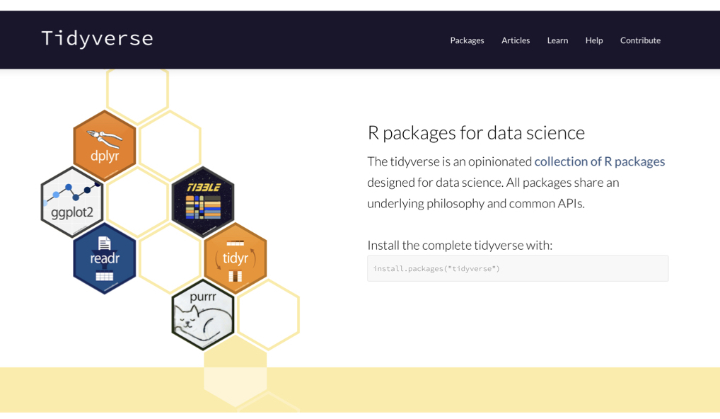
Core Tidyverse Packages
The core packages are listed in Table 14.1; ggplot2 has its own chapter (Chapter 13) and purrr is used in Chapter 15.
| Package | Purpose | pandas / Python equivalent |
|---|---|---|
| dplyr | Data manipulation (filter, select, mutate, etc.) | pandas methods: .query(), .assign(), .groupby()
|
| ggplot2 | Data visualization | matplotlib / seaborn / plotnine |
| tidyr | Data tidying (pivot, separate, etc.) |
.melt(), .pivot()
|
| readr | Fast data import | pd.read_csv() |
| purrr | Functional programming | list comprehensions |
| stringr | String manipulation |
str methods, re
|
| forcats | Working with factors | pd.Categorical |
| tibble | Modern data frames | pd.DataFrame |
Load all core packages at once with a single library() call:
This loads the core tidyverse packages and displays helpful information about function conflicts (Wickham et al., 2019). For example, the message notes that dplyr::filter() masks stats::filter(): once the tidyverse is loaded, typing filter() gives you the dplyr version, and you must write stats::filter() to reach the base R one (Section 11.9.3).
Data Import with readr
The readr package provides fast, friendly functions for reading rectangular data. It’s more consistent and feature-rich than base R’s read.csv().
# Basic CSV import (tidyverse alternative to read.csv)
data <- read_csv("experiment_results.csv")

# Tab-separated files
data <- read_tsv("data.tsv")

# Semicolon-separated (common in European locales)
data <- read_csv2("data.csv")

# Fixed-width files
data <- read_fwf("data.txt", fwf_widths(c(10, 5, 8)))
Controlling Column Types
By default, read_csv() guesses column types from the first 1000 rows. You can override this with col_types:
# Specify column types explicitly
data <- read_csv(
  "samples.csv",
  col_types = cols(
    sample_id = col_character(),    # Force as character
    count = col_integer(),          # Integer values
    concentration = col_double(),   # Decimal numbers
    date = col_date(),              # Parse as date
    treatment = col_factor(levels = c("control", "drug_A", "drug_B"))
  )
)

# Shorthand specification (c = character, i = integer, d = double, D = date)
data <- read_csv("samples.csv", col_types = "ciidD")

# Only override specific columns, guess the rest
data <- read_csv(
  "samples.csv",
  col_types = cols(
    sample_id = col_character(),
    .default = col_guess()
  )
)Always check problems(data) after reading to see if any values couldn’t be parsed as expected. This catches data quality issues early!
Handling Messy Column Names
Real-world data often has problematic column names (spaces, special characters, inconsistent capitalization). The janitor package provides clean_names() to standardize them:
This converts all names to lowercase snake_case, making them valid R identifiers and consistent to work with.
14.2 The Pipe Operator
One of the most powerful features of the tidyverse is the pipe operator, which allows you to chain operations together in a readable way. The pipe passes the result of one operation as the first argument of the next (Figure 14.2). Read it as “then”: take the data, then filter, then group, then summarize. This left-to-right, top-to-bottom flow mirrors how we think about data transformations, and it is the same idea as the Unix pipe | from Section 7.6, applied to R objects instead of text streams.
The Native Pipe: |>
R 4.1+ includes a native pipe operator |>:
The magrittr Pipe: %>%
The tidyverse also provides %>% from the magrittr package, which predates the native pipe and is what you will see in older code and tutorials:
The two differ in small ways: %>% uses . as a placeholder for the piped value and lets you call a function without parentheses (x %>% mean), while |> uses _ as a placeholder (only for a named argument) and always requires parentheses. |> needs no package, so this book uses it throughout; either is fine as long as you are consistent within a project.
The pipe transforms x |> f(y) into f(x, y). Think of it as “take this, then do that.” This makes code read like a recipe: take data, then filter, then select, then summarize. In Positron and RStudio, Ctrl/Cmd + Shift + M inserts a pipe (Appendix A).
14.3 Data Manipulation with dplyr
The dplyr package provides a consistent set of “verbs” for data manipulation. These functions are designed to be intuitive and compose well together.
The Five Core dplyr Verbs
Table 14.2 summarizes the five verbs; the same verbs work on database tables through dbplyr (Chapter 22).
| Verb | Action |
|---|---|
filter() |
Pick rows based on conditions |
select() |
Pick columns by name |
arrange() |
Reorder rows |
mutate() |
Create or modify columns |
summarize() |
Reduce to summary statistics |
Let’s create sample data to demonstrate these:
# Sample experimental data
experiments <- tibble(
  sample_id = paste0("S", 1:12),
  treatment = rep(c("control", "drug_A", "drug_B"), each = 4),
  replicate = rep(1:4, 3),
  expression = c(10.2, 11.1, 9.8, 10.5,   # control
                 15.3, 14.8, 16.2, 15.0,   # drug_A
                 18.1, 19.2, 17.5, 18.8),  # drug_B
  cell_count = c(1000, 1050, 980, 1020,
                 1100, 1080, 1150, 1090,
                 1200, 1250, 1180, 1220)
)

experiments| sample_id | treatment | replicate | expression | cell_count |
|---|---|---|---|---|
| S1 | control | 1 | 10.2 | 1000 |
| S2 | control | 2 | 11.1 | 1050 |
| S3 | control | 3 | 9.8 | 980 |
| S4 | control | 4 | 10.5 | 1020 |
| S5 | drug_A | 1 | 15.3 | 1100 |
| S6 | drug_A | 2 | 14.8 | 1080 |
| S7 | drug_A | 3 | 16.2 | 1150 |
| S8 | drug_A | 4 | 15.0 | 1090 |
| S9 | drug_B | 1 | 18.1 | 1200 |
| S10 | drug_B | 2 | 19.2 | 1250 |
| S11 | drug_B | 3 | 17.5 | 1180 |
| S12 | drug_B | 4 | 18.8 | 1220 |
Filtering Rows with filter()
Select rows that meet specific conditions:
| sample_id | treatment | replicate | expression | cell_count |
|---|---|---|---|---|
| S5 | drug_A | 1 | 15.3 | 1100 |
| S6 | drug_A | 2 | 14.8 | 1080 |
| S7 | drug_A | 3 | 16.2 | 1150 |
| S8 | drug_A | 4 | 15.0 | 1090 |
| sample_id | treatment | replicate | expression | cell_count |
|---|---|---|---|---|
| S5 | drug_A | 1 | 15.3 | 1100 |
| S7 | drug_A | 3 | 16.2 | 1150 |
| sample_id | treatment | replicate | expression | cell_count |
|---|---|---|---|---|
| S5 | drug_A | 1 | 15.3 | 1100 |
| S6 | drug_A | 2 | 14.8 | 1080 |
| S7 | drug_A | 3 | 16.2 | 1150 |
| S8 | drug_A | 4 | 15.0 | 1090 |
| S9 | drug_B | 1 | 18.1 | 1200 |
| S10 | drug_B | 2 | 19.2 | 1250 |
| S11 | drug_B | 3 | 17.5 | 1180 |
| S12 | drug_B | 4 | 18.8 | 1220 |
| sample_id | treatment | replicate | expression | cell_count |
|---|---|---|---|---|
| S5 | drug_A | 1 | 15.3 | 1100 |
| S6 | drug_A | 2 | 14.8 | 1080 |
| S7 | drug_A | 3 | 16.2 | 1150 |
| S8 | drug_A | 4 | 15.0 | 1090 |
| S9 | drug_B | 1 | 18.1 | 1200 |
| S10 | drug_B | 2 | 19.2 | 1250 |
| S11 | drug_B | 3 | 17.5 | 1180 |
| S12 | drug_B | 4 | 18.8 | 1220 |
Conditions are built from the comparison and logical operators in Table 14.3 (see Section 11.7.3). Separate conditions with commas for AND; & and | combine conditions the way set intersection and union do (Figure 14.3).
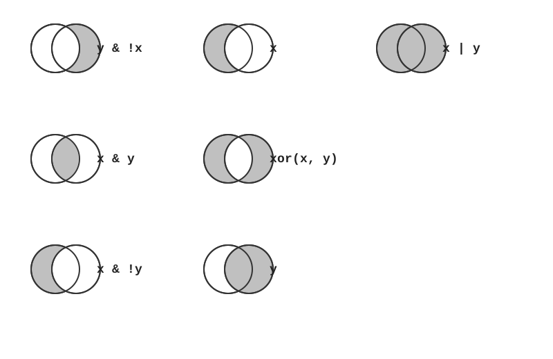
& keeps rows in both sets, | keeps rows in either, and ! keeps the complement.
filter() keeps only rows where the condition is TRUE. Rows where the condition evaluates to NA are silently dropped, so filter(expression > 15) also removes rows with a missing expression. Use is.na() explicitly if you want to keep or inspect them (Section 14.4).
Selecting Columns with select()
Choose which columns to keep:
| sample_id | treatment | expression |
|---|---|---|
| S1 | control | 10.2 |
| S2 | control | 11.1 |
| S3 | control | 9.8 |
| S4 | control | 10.5 |
| S5 | drug_A | 15.3 |
| S6 | drug_A | 14.8 |
| S7 | drug_A | 16.2 |
| S8 | drug_A | 15.0 |
| S9 | drug_B | 18.1 |
| S10 | drug_B | 19.2 |
| S11 | drug_B | 17.5 |
| S12 | drug_B | 18.8 |
| sample_id | treatment | replicate |
|---|---|---|
| S1 | control | 1 |
| S2 | control | 2 |
| S3 | control | 3 |
| S4 | control | 4 |
| S5 | drug_A | 1 |
| S6 | drug_A | 2 |
| S7 | drug_A | 3 |
| S8 | drug_A | 4 |
| S9 | drug_B | 1 |
| S10 | drug_B | 2 |
| S11 | drug_B | 3 |
| S12 | drug_B | 4 |
| sample_id | treatment | replicate | expression |
|---|---|---|---|
| S1 | control | 1 | 10.2 |
| S2 | control | 2 | 11.1 |
| S3 | control | 3 | 9.8 |
| S4 | control | 4 | 10.5 |
| S5 | drug_A | 1 | 15.3 |
| S6 | drug_A | 2 | 14.8 |
| S7 | drug_A | 3 | 16.2 |
| S8 | drug_A | 4 | 15.0 |
| S9 | drug_B | 1 | 18.1 |
| S10 | drug_B | 2 | 19.2 |
| S11 | drug_B | 3 | 17.5 |
| S12 | drug_B | 4 | 18.8 |
| expression |
|---|
| 10.2 |
| 11.1 |
| 9.8 |
| 10.5 |
| 15.3 |
| 14.8 |
| 16.2 |
| 15.0 |
| 18.1 |
| 19.2 |
| 17.5 |
| 18.8 |
| replicate | expression | cell_count |
|---|---|---|
| 1 | 10.2 | 1000 |
| 2 | 11.1 | 1050 |
| 3 | 9.8 | 980 |
| 4 | 10.5 | 1020 |
| 1 | 15.3 | 1100 |
| 2 | 14.8 | 1080 |
| 3 | 16.2 | 1150 |
| 4 | 15.0 | 1090 |
| 1 | 18.1 | 1200 |
| 2 | 19.2 | 1250 |
| 3 | 17.5 | 1180 |
| 4 | 18.8 | 1220 |
| expression | cell_count | sample_id | treatment | replicate |
|---|---|---|---|---|
| 10.2 | 1000 | S1 | control | 1 |
| 11.1 | 1050 | S2 | control | 2 |
| 9.8 | 980 | S3 | control | 3 |
| 10.5 | 1020 | S4 | control | 4 |
| 15.3 | 1100 | S5 | drug_A | 1 |
| 14.8 | 1080 | S6 | drug_A | 2 |
| 16.2 | 1150 | S7 | drug_A | 3 |
| 15.0 | 1090 | S8 | drug_A | 4 |
| 18.1 | 1200 | S9 | drug_B | 1 |
| 19.2 | 1250 | S10 | drug_B | 2 |
| 17.5 | 1180 | S11 | drug_B | 3 |
| 18.8 | 1220 | S12 | drug_B | 4 |
The selection helpers are useful with wide datasets: starts_with(), ends_with(), and contains() match literal text, matches() takes a regular expression (Chapter 9), num_range("x", 1:3) picks x1, x2, x3, where() selects by a predicate on the column, and everything() stands for all remaining columns (handy for reordering). The same helpers work inside pivot_longer() and across().
Arranging Rows with arrange()
Sort data by one or more columns:
| sample_id | treatment | replicate | expression | cell_count |
|---|---|---|---|---|
| S3 | control | 3 | 9.8 | 980 |
| S1 | control | 1 | 10.2 | 1000 |
| S4 | control | 4 | 10.5 | 1020 |
| S2 | control | 2 | 11.1 | 1050 |
| S6 | drug_A | 2 | 14.8 | 1080 |
| S8 | drug_A | 4 | 15.0 | 1090 |
| S5 | drug_A | 1 | 15.3 | 1100 |
| S7 | drug_A | 3 | 16.2 | 1150 |
| S11 | drug_B | 3 | 17.5 | 1180 |
| S9 | drug_B | 1 | 18.1 | 1200 |
| S12 | drug_B | 4 | 18.8 | 1220 |
| S10 | drug_B | 2 | 19.2 | 1250 |
| sample_id | treatment | replicate | expression | cell_count |
|---|---|---|---|---|
| S10 | drug_B | 2 | 19.2 | 1250 |
| S12 | drug_B | 4 | 18.8 | 1220 |
| S9 | drug_B | 1 | 18.1 | 1200 |
| S11 | drug_B | 3 | 17.5 | 1180 |
| S7 | drug_A | 3 | 16.2 | 1150 |
| S5 | drug_A | 1 | 15.3 | 1100 |
| S8 | drug_A | 4 | 15.0 | 1090 |
| S6 | drug_A | 2 | 14.8 | 1080 |
| S2 | control | 2 | 11.1 | 1050 |
| S4 | control | 4 | 10.5 | 1020 |
| S1 | control | 1 | 10.2 | 1000 |
| S3 | control | 3 | 9.8 | 980 |
| sample_id | treatment | replicate | expression | cell_count |
|---|---|---|---|---|
| S2 | control | 2 | 11.1 | 1050 |
| S4 | control | 4 | 10.5 | 1020 |
| S1 | control | 1 | 10.2 | 1000 |
| S3 | control | 3 | 9.8 | 980 |
| S7 | drug_A | 3 | 16.2 | 1150 |
| S5 | drug_A | 1 | 15.3 | 1100 |
| S8 | drug_A | 4 | 15.0 | 1090 |
| S6 | drug_A | 2 | 14.8 | 1080 |
| S10 | drug_B | 2 | 19.2 | 1250 |
| S12 | drug_B | 4 | 18.8 | 1220 |
| S9 | drug_B | 1 | 18.1 | 1200 |
| S11 | drug_B | 3 | 17.5 | 1180 |
Missing values are always sorted to the end, regardless of whether you sort ascending or descending.
Creating Columns with mutate()
Add new columns or modify existing ones:
| sample_id | treatment | replicate | expression | cell_count | log_expression | expression_per_cell |
|---|---|---|---|---|---|---|
| S1 | CONTROL | 1 | 10.2 | 1000 | 3.350497 | 10.20000 |
| S2 | CONTROL | 2 | 11.1 | 1050 | 3.472488 | 10.57143 |
| S3 | CONTROL | 3 | 9.8 | 980 | 3.292782 | 10.00000 |
| S4 | CONTROL | 4 | 10.5 | 1020 | 3.392317 | 10.29412 |
| S5 | DRUG_A | 1 | 15.3 | 1100 | 3.935460 | 13.90909 |
| S6 | DRUG_A | 2 | 14.8 | 1080 | 3.887525 | 13.70370 |
| S7 | DRUG_A | 3 | 16.2 | 1150 | 4.017922 | 14.08696 |
| S8 | DRUG_A | 4 | 15.0 | 1090 | 3.906891 | 13.76147 |
| S9 | DRUG_B | 1 | 18.1 | 1200 | 4.177918 | 15.08333 |
| S10 | DRUG_B | 2 | 19.2 | 1250 | 4.263034 | 15.36000 |
| S11 | DRUG_B | 3 | 17.5 | 1180 | 4.129283 | 14.83051 |
| S12 | DRUG_B | 4 | 18.8 | 1220 | 4.232661 | 15.40984 |
New columns can refer to columns created earlier in the same mutate() call. Any vectorized function works inside mutate(); the ones you will reach for most often are:
- Arithmetic (
+,-,*,/,^) and modular arithmetic (%/%,%%) - Logs and roots:
log(),log2(),log10(),sqrt() - Offsets:
lead(),lag()(Section 11.18.2) - Cumulative aggregates:
cumsum(),cummax(),cummean()(Section 11.18.1) - Ranking:
min_rank(),dense_rank(),row_number()(Section 11.18.3) - Conditionals:
if_else()(Section 11.16.2) andcase_when()(Section 14.6.1)
Replacing Columns with transmute()
If you only want to keep the new columns (discarding all others), use transmute():
| sample_id | log_expression | normalized |
|---|---|---|
| S1 | 3.350497 | 10.20000 |
| S2 | 3.472488 | 10.57143 |
| S3 | 3.292782 | 10.00000 |
| S4 | 3.392317 | 10.29412 |
| S5 | 3.935460 | 13.90909 |
| S6 | 3.887525 | 13.70370 |
| S7 | 4.017922 | 14.08696 |
| S8 | 3.906891 | 13.76147 |
| S9 | 4.177918 | 15.08333 |
| S10 | 4.263034 | 15.36000 |
| S11 | 4.129283 | 14.83051 |
| S12 | 4.232661 | 15.40984 |
This is useful when you’re creating a derived dataset and don’t need the original columns.
Summarizing Data with summarize()
Collapse multiple rows into summary statistics (summarise(), with the British spelling, is an identical alias):
| mean_expression | sd_expression | n_samples |
|---|---|---|
| 14.70833 | 3.490626 | 12 |
Common summary functions include mean(), median(), sd(), var(), IQR(), min(), max(), quantile(), first(), last(), nth(), n(), and n_distinct().
Aggregation functions return NA if any input value is NA. Pass na.rm = TRUE (for example mean(expression, na.rm = TRUE)) to drop missing values before computing, or handle them explicitly first (Section 14.4).
Grouping with group_by()
The real power of summarize() comes with group_by():
| treatment | mean_expression | sd_expression | n |
|---|---|---|---|
| control | 10.400 | 0.5477226 | 4 |
| drug_A | 15.325 | 0.6184658 | 4 |
| drug_B | 18.400 | 0.7527727 | 4 |
| treatment | mean_expr | max_expr | min_expr |
|---|---|---|---|
| drug_B | 18.400 | 19.2 | 17.5 |
| drug_A | 15.325 | 16.2 | 14.8 |
| control | 10.400 | 11.1 | 9.8 |
You can group by more than one variable, and grouping affects mutate() as well as summarize(): inside a grouped mutate(), functions like mean() or min_rank() are computed within each group, which is how you centre values on their group mean or rank samples within a treatment.
| sample_id | treatment | replicate | expression | cell_count | rank_in_group | expr_vs_group_mean |
|---|---|---|---|---|---|---|
| S1 | control | 1 | 10.2 | 1000 | 3 | -0.200 |
| S2 | control | 2 | 11.1 | 1050 | 1 | 0.700 |
| S3 | control | 3 | 9.8 | 980 | 4 | -0.600 |
| S4 | control | 4 | 10.5 | 1020 | 2 | 0.100 |
| S5 | drug_A | 1 | 15.3 | 1100 | 2 | -0.025 |
| S6 | drug_A | 2 | 14.8 | 1080 | 4 | -0.525 |
| S7 | drug_A | 3 | 16.2 | 1150 | 1 | 0.875 |
| S8 | drug_A | 4 | 15.0 | 1090 | 3 | -0.325 |
| S9 | drug_B | 1 | 18.1 | 1200 | 3 | -0.300 |
| S10 | drug_B | 2 | 19.2 | 1250 | 1 | 0.800 |
| S11 | drug_B | 3 | 17.5 | 1180 | 4 | -0.900 |
| S12 | drug_B | 4 | 18.8 | 1220 | 2 | 0.400 |
Three things to know about grouped data frames:
- A grouped tibble prints its groups at the top (
# Groups: treatment [3]), and every later verb respects the grouping until you remove it -
summarize()peels off one level of grouping, so after grouping by two variables the result is still grouped by the first. Pass.groups = "drop"to return an ungrouped result, or callungroup() - Forgetting to
ungroup()is a common source of surprising results later in a pipeline; make it a habit to ungroup as soon as the grouped step is done
Chaining Operations Together
The power of dplyr shines when chaining multiple operations:
| treatment | mean_log_expr | se |
|---|---|---|
| drug_B | 4.200724 | 0.0296177 |
| drug_A | 3.936949 | 0.0287301 |
14.4 Handling Missing Values
Missing values are ubiquitous in real data. R represents them as NA (Section 11.7.2), and most operations involving NA return NA, which is deliberate: R refuses to guess. Wrangling therefore usually starts by finding out where the missing values are and deciding what to do with them.
Detecting Missing Values
is.na() returns TRUE for each missing value; summing it counts them.
# A dataset with some gaps
assays <- tibble(
  sample_id = paste0("S", 1:6),
  treatment = c("control", "control", "drug_A", "drug_A", "drug_B", NA),
  expression = c(10.2, NA, 15.3, 14.8, NA, 18.1)
)

# Any missing at all?
any(is.na(assays))
#> [1] TRUE

# Count missing values per column
assays |>
summarize(across(everything(), \(x) sum(is.na(x))))| sample_id | treatment | expression |
|---|---|---|
| 0 | 1 | 2 |
across() applies the same function to several columns at once; it is the tidyverse’s general tool for “do this to every column that …”, and it takes the same selection helpers as select().
Dropping Rows with Missing Values
| sample_id | treatment | expression |
|---|---|---|
| S1 | control | 10.2 |
| S3 | drug_A | 15.3 |
| S4 | drug_A | 14.8 |
| S6 | NA | 18.1 |
| sample_id | treatment | expression |
|---|---|---|
| S1 | control | 10.2 |
| S3 | drug_A | 15.3 |
| S4 | drug_A | 14.8 |
| S6 | NA | 18.1 |
| sample_id | treatment | expression |
|---|---|---|
| S1 | control | 10.2 |
| S3 | drug_A | 15.3 |
| S4 | drug_A | 14.8 |
Replacing Missing Values
Sometimes a missing value has a known meaning (a count that was not recorded because nothing was found, for instance) and should be replaced rather than dropped:
| sample_id | treatment | expression |
|---|---|---|
| S1 | control | 10.2 |
| S2 | control | NA |
| S3 | drug_A | 15.3 |
| S4 | drug_A | 14.8 |
| S5 | drug_B | NA |
| S6 | unknown | 18.1 |
| sample_id | treatment | expression |
|---|---|---|
| S1 | control | 10.2 |
| S2 | control | 0.0 |
| S3 | drug_A | 15.3 |
| S4 | drug_A | 14.8 |
| S5 | drug_B | 0.0 |
| S6 | unknown | 18.1 |
| sample_id | treatment | expression |
|---|---|---|
| S1 | control | 10.2 |
| S2 | control | 14.6 |
| S3 | drug_A | 15.3 |
| S4 | drug_A | 14.8 |
| S5 | drug_B | 14.6 |
| S6 | NA | 18.1 |
Never blindly drop or fill missing values. Ask why they are missing: an assay that failed at random is different from values that are missing because they fell below a detection limit. The pattern of missingness determines whether dropping, replacing, or flagging (mutate(expr_missing = is.na(expression))) is the right choice.
14.5 Tibbles: Modern Data Frames
Tibbles are the tidyverse’s enhanced version of data frames (Figure 14.4). They are designed to be more consistent and more informative than the base data frames of Section 11.10, while remaining compatible with almost everything that works on a data frame.
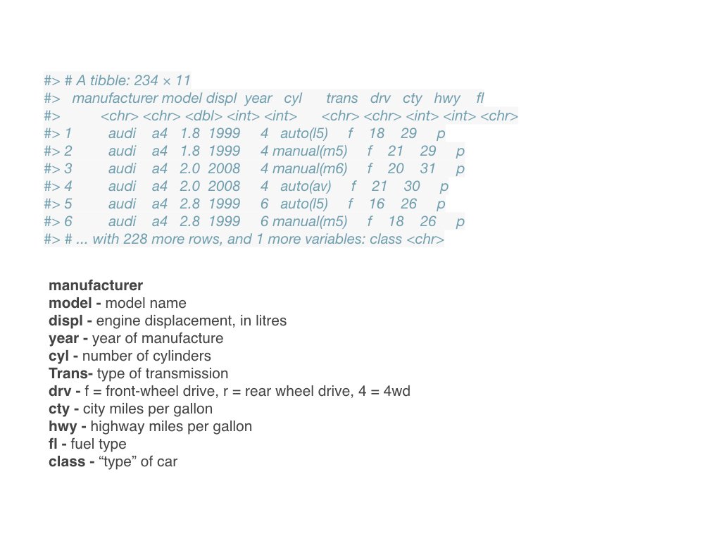
Creating Tibbles
| x | y | z |
|---|---|---|
| 1 | 1 | a |
| 2 | 4 | b |
| 3 | 9 | c |
| 4 | 16 | d |
| 5 | 25 | e |
| mpg | cyl | disp | hp | drat | wt | qsec | vs | am | gear | carb |
|---|---|---|---|---|---|---|---|---|---|---|
| 21.0 | 6 | 160 | 110 | 3.90 | 2.620 | 16.46 | 0 | 1 | 4 | 4 |
| 21.0 | 6 | 160 | 110 | 3.90 | 2.875 | 17.02 | 0 | 1 | 4 | 4 |
| 22.8 | 4 | 108 | 93 | 3.85 | 2.320 | 18.61 | 1 | 1 | 4 | 1 |
| 21.4 | 6 | 258 | 110 | 3.08 | 3.215 | 19.44 | 1 | 0 | 3 | 1 |
| 18.7 | 8 | 360 | 175 | 3.15 | 3.440 | 17.02 | 0 | 0 | 3 | 2 |
| 18.1 | 6 | 225 | 105 | 2.76 | 3.460 | 20.22 | 1 | 0 | 3 | 1 |
Creating Small Tibbles with tribble()
For small datasets (especially examples or test data), tribble() provides a row-by-row format that’s easier to read:
| sample_id | treatment | expression |
|---|---|---|
| S001 | control | 10.2 |
| S002 | drug_A | 15.3 |
| S003 | drug_B | 18.1 |
This format is particularly useful for:
- Creating examples in documentation
- Quick test datasets
- Small lookup tables
Inspecting Tibbles
Printing a tibble shows its dimensions, the first 10 rows, only as many columns as fit on screen, and the type of each column in angle brackets under its name (Table 14.4).
| Abbreviation | Column type |
|---|---|
<chr> |
character |
<dbl> |
double (numeric with decimals) |
<int> |
integer |
<lgl> |
logical |
<fct> |
factor |
<date> |
Date |
<dttm> |
date-time |
For a dataset with many columns, glimpse() gives a transposed view with one line per column, showing its type and first few values; it is usually the first thing to run on newly imported data. The base R functions from Section 11.10.2 (dim(), nrow(), names(), str(), summary()) all work on tibbles too.
glimpse(as_tibble(mtcars))
#> Rows: 32
#> Columns: 11
#> $ mpg  <dbl> 21.0, 21.0, 22.8, 21.4, 18.7, 18.1, 14.3, 24.4, 22.8, 19.2, 17.8,…
#> $ cyl  <dbl> 6, 6, 4, 6, 8, 6, 8, 4, 4, 6, 6, 8, 8, 8, 8, 8, 8, 4, 4, 4, 4, 8,…
#> $ disp <dbl> 160.0, 160.0, 108.0, 258.0, 360.0, 225.0, 360.0, 146.7, 140.8, 16…
#> $ hp   <dbl> 110, 110, 93, 110, 175, 105, 245, 62, 95, 123, 123, 180, 180, 180…
#> $ drat <dbl> 3.90, 3.90, 3.85, 3.08, 3.15, 2.76, 3.21, 3.69, 3.92, 3.92, 3.92,…
#> $ wt   <dbl> 2.620, 2.875, 2.320, 3.215, 3.440, 3.460, 3.570, 3.190, 3.150, 3.…
#> $ qsec <dbl> 16.46, 17.02, 18.61, 19.44, 17.02, 20.22, 15.84, 20.00, 22.90, 18…
#> $ vs   <dbl> 0, 0, 1, 1, 0, 1, 0, 1, 1, 1, 1, 0, 0, 0, 0, 0, 0, 1, 1, 1, 1, 0,…
#> $ am   <dbl> 1, 1, 1, 0, 0, 0, 0, 0, 0, 0, 0, 0, 0, 0, 0, 0, 0, 1, 1, 1, 0, 0,…
#> $ gear <dbl> 4, 4, 4, 3, 3, 3, 3, 4, 4, 4, 4, 3, 3, 3, 3, 3, 3, 4, 4, 4, 3, 3,…
#> $ carb <dbl> 4, 4, 1, 1, 2, 1, 4, 2, 2, 4, 4, 3, 3, 3, 4, 4, 4, 1, 2, 1, 1, 2,…

# Extract a column as a vector
my_tibble$z
#> [1] "a" "b" "c" "d" "e"
my_tibble[["z"]]
#> [1] "a" "b" "c" "d" "e"
Tibble Advantages
- Better printing: Shows first 10 rows, fits columns to screen, and reports column types
-
No partial matching:
df$colwon’t matchdf$column, and accessing a column that does not exist gives a warning - No string-to-factor conversion: Characters stay as characters
-
Preserves column types: Subsetting with
[always returns a tibble -
No row names: Anything meaningful belongs in a proper column (use
rownames_to_column()when converting a data frame such asmtcars)
# Data frame subsetting can surprise you
df <- data.frame(x = 1:3, y = 4:6)
class(df[, 1])  # Returns vector!
#> [1] "integer"

# Tibble subsetting is consistent
tb <- tibble(x = 1:3, y = 4:6)
class(tb[, 1])  # Returns tibble
#> [1] "tbl_df"     "tbl"        "data.frame"

# Row names become a column
mtcars |>
  rownames_to_column("car") |>
  as_tibble() |>
head(3)| car | mpg | cyl | disp | hp | drat | wt | qsec | vs | am | gear | carb |
|---|---|---|---|---|---|---|---|---|---|---|---|
| Mazda RX4 | 21.0 | 6 | 160 | 110 | 3.90 | 2.620 | 16.46 | 0 | 1 | 4 | 4 |
| Mazda RX4 Wag | 21.0 | 6 | 160 | 110 | 3.90 | 2.875 | 17.02 | 0 | 1 | 4 | 4 |
| Datsun 710 | 22.8 | 4 | 108 | 93 | 3.85 | 2.320 | 18.61 | 1 | 1 | 4 | 1 |
14.6 Additional dplyr Functions
Conditional Logic with case_when()
| sample_id | treatment | replicate | expression | cell_count | expression_level |
|---|---|---|---|---|---|
| S1 | control | 1 | 10.2 | 1000 | low |
| S2 | control | 2 | 11.1 | 1050 | low |
| S3 | control | 3 | 9.8 | 980 | low |
| S4 | control | 4 | 10.5 | 1020 | low |
| S5 | drug_A | 1 | 15.3 | 1100 | medium |
| S6 | drug_A | 2 | 14.8 | 1080 | medium |
| S7 | drug_A | 3 | 16.2 | 1150 | medium |
| S8 | drug_A | 4 | 15.0 | 1090 | medium |
| S9 | drug_B | 1 | 18.1 | 1200 | high |
| S10 | drug_B | 2 | 19.2 | 1250 | high |
| S11 | drug_B | 3 | 17.5 | 1180 | high |
| S12 | drug_B | 4 | 18.8 | 1220 | high |
Counting with count()
| treatment | n |
|---|---|
| control | 4 |
| drug_A | 4 |
| drug_B | 4 |
| treatment | n |
|---|---|
| control | 4 |
| drug_A | 4 |
| drug_B | 4 |
| treatment | late_replicate | n |
|---|---|---|
| control | FALSE | 2 |
| control | TRUE | 2 |
| drug_A | FALSE | 2 |
| drug_A | TRUE | 2 |
| drug_B | FALSE | 2 |
| drug_B | TRUE | 2 |
| treatment | n |
|---|---|
| control | 4050 |
| drug_A | 4420 |
| drug_B | 4850 |
You can also use n_distinct() within summarize() to count unique values:
| n_samples | n_treatments | n_replicates |
|---|---|---|
| 12 | 3 | 4 |
| treatment | samples | unique_replicates |
|---|---|---|
| control | 4 | 4 |
| drug_A | 4 | 4 |
| drug_B | 4 | 4 |
Distinct Values with distinct()
| treatment |
|---|
| control |
| drug_A |
| drug_B |
| treatment | late_replicate |
|---|---|
| control | FALSE |
| control | TRUE |
| drug_A | FALSE |
| drug_A | TRUE |
| drug_B | FALSE |
| drug_B | TRUE |
| sample_id | treatment | replicate | expression | cell_count |
|---|---|---|---|---|
| S1 | control | 1 | 10.2 | 1000 |
| S5 | drug_A | 1 | 15.3 | 1100 |
| S9 | drug_B | 1 | 18.1 | 1200 |
With no column names, distinct() removes exactly duplicated rows. Checking for duplicates is a standard data-quality step after import: any(duplicated(df)) tells you whether any exist, df[duplicated(df), ] shows them, and distinct(df) removes them.
Renaming with rename()
| sample_id | treatment | replicate | expr | cells |
|---|---|---|---|---|
| S1 | control | 1 | 10.2 | 1000 |
| S2 | control | 2 | 11.1 | 1050 |
| S3 | control | 3 | 9.8 | 980 |
| S4 | control | 4 | 10.5 | 1020 |
| S5 | drug_A | 1 | 15.3 | 1100 |
| S6 | drug_A | 2 | 14.8 | 1080 |
| S7 | drug_A | 3 | 16.2 | 1150 |
| S8 | drug_A | 4 | 15.0 | 1090 |
| S9 | drug_B | 1 | 18.1 | 1200 |
| S10 | drug_B | 2 | 19.2 | 1250 |
| S11 | drug_B | 3 | 17.5 | 1180 |
| S12 | drug_B | 4 | 18.8 | 1220 |
Subsetting Rows with slice()
While filter() selects rows based on conditions, slice() selects rows by position:
| sample_id | treatment | replicate | expression | cell_count |
|---|---|---|---|---|
| S1 | control | 1 | 10.2 | 1000 |
| S2 | control | 2 | 11.1 | 1050 |
| S3 | control | 3 | 9.8 | 980 |
| sample_id | treatment | replicate | expression | cell_count |
|---|---|---|---|---|
| S11 | drug_B | 3 | 17.5 | 1180 |
| S12 | drug_B | 4 | 18.8 | 1220 |
| sample_id | treatment | replicate | expression | cell_count |
|---|---|---|---|---|
| S1 | control | 1 | 10.2 | 1000 |
| S5 | drug_A | 1 | 15.3 | 1100 |
| S12 | drug_B | 4 | 18.8 | 1220 |
| sample_id | treatment | replicate | expression | cell_count |
|---|---|---|---|---|
| S10 | drug_B | 2 | 19.2 | 1250 |
| S12 | drug_B | 4 | 18.8 | 1220 |
| S9 | drug_B | 1 | 18.1 | 1200 |
| sample_id | treatment | replicate | expression | cell_count |
|---|---|---|---|---|
| S9 | drug_B | 1 | 18.1 | 1200 |
| S10 | drug_B | 2 | 19.2 | 1250 |
| S4 | control | 4 | 10.5 | 1020 |
| sample_id | treatment | replicate | expression | cell_count |
|---|---|---|---|---|
| S2 | control | 2 | 11.1 | 1050 |
| S7 | drug_A | 3 | 16.2 | 1150 |
| S10 | drug_B | 2 | 19.2 | 1250 |
Extracting Columns with pull()
To extract a single column as a vector (rather than a data frame), use pull():
14.7 Working with Factors
Factors are R’s way of representing categorical data with a fixed set of possible values (called levels). The forcats package (part of the tidyverse) provides tools for working with factors.
Creating and Inspecting Factors
Reordering Factor Levels
For visualization (Section 13.9.3), you often want to order factor levels meaningfully:
library(forcats)

# Sample data
gene_data <- tibble(
  gene = c("BRCA1", "TP53", "EGFR", "KRAS", "MYC"),
  expression = c(5.2, 8.1, 3.4, 6.7, 9.2)
)

# Reorder gene by expression for better plotting
gene_data |>
  mutate(gene = fct_reorder(gene, expression)) |>
  ggplot(aes(x = expression, y = gene)) +
  geom_point(size = 3) +
  labs(title = "Gene Expression (ordered)")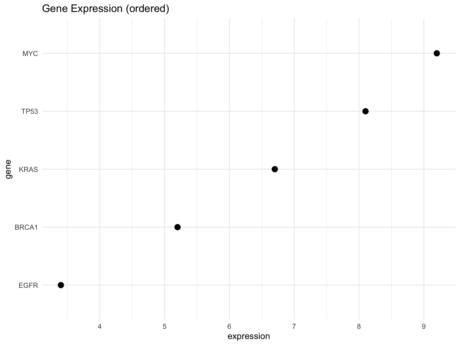
fct_reorder() so the plot reads from lowest to highest
Other useful reordering functions:
-
fct_infreq(): Order by frequency (most common first) -
fct_rev(): Reverse the order -
fct_relevel(): Manually move specific levels to the front
Recoding Factor Levels
Use fct_recode() to change level names:
Collapsing Factor Levels
Use fct_collapse() to combine multiple levels into one:
# Combine related categories
tissue <- factor(c("brain", "liver", "heart", "kidney", "lung", "spleen"))

fct_collapse(tissue,
  neural = "brain",
  digestive = "liver",
  circulatory = c("heart", "lung"),
  other = c("kidney", "spleen")
)
#> [1] neural      digestive   circulatory other       circulatory other
#> Levels: neural circulatory other digestive
Lumping Rare Levels
Use fct_lump_*() functions to combine rare categories into “Other”:
# Sample with many categories
samples <- factor(rep(c("A", "B", "C", "D", "E", "F"), c(50, 30, 10, 5, 3, 2)))

# Keep only the top 3 most common
fct_lump_n(samples, n = 3)
#>   [1] A     A     A     A     A     A     A     A     A     A     A     A
#>  [13] A     A     A     A     A     A     A     A     A     A     A     A
#>  [25] A     A     A     A     A     A     A     A     A     A     A     A
#>  [37] A     A     A     A     A     A     A     A     A     A     A     A
#>  [49] A     A     B     B     B     B     B     B     B     B     B     B
#>  [61] B     B     B     B     B     B     B     B     B     B     B     B
#>  [73] B     B     B     B     B     B     B     B     C     C     C     C
#>  [85] C     C     C     C     C     C     Other Other Other Other Other Other
#>  [97] Other Other Other Other
#> Levels: A B C Other

# Keep levels that appear at least 10 times
fct_lump_min(samples, min = 10)
#>   [1] A     A     A     A     A     A     A     A     A     A     A     A
#>  [13] A     A     A     A     A     A     A     A     A     A     A     A
#>  [25] A     A     A     A     A     A     A     A     A     A     A     A
#>  [37] A     A     A     A     A     A     A     A     A     A     A     A
#>  [49] A     A     B     B     B     B     B     B     B     B     B     B
#>  [61] B     B     B     B     B     B     B     B     B     B     B     B
#>  [73] B     B     B     B     B     B     B     B     C     C     C     C
#>  [85] C     C     C     C     C     C     Other Other Other Other Other Other
#>  [97] Other Other Other Other
#> Levels: A B C Other

# Lump levels that make up less than 5% of the data
fct_lump_prop(samples, prop = 0.05)
#>   [1] A     A     A     A     A     A     A     A     A     A     A     A
#>  [13] A     A     A     A     A     A     A     A     A     A     A     A
#>  [25] A     A     A     A     A     A     A     A     A     A     A     A
#>  [37] A     A     A     A     A     A     A     A     A     A     A     A
#>  [49] A     A     B     B     B     B     B     B     B     B     B     B
#>  [61] B     B     B     B     B     B     B     B     B     B     B     B
#>  [73] B     B     B     B     B     B     B     B     C     C     C     C
#>  [85] C     C     C     C     C     C     Other Other Other Other Other Other
#>  [97] Other Other Other Other
#> Levels: A B C OtherWhen plotting categorical data, proper factor ordering makes visualizations much easier to read. Always consider whether alphabetical order (the default) or a data-driven order (by value, frequency) is more meaningful.
14.8 Joining Data Frames
In real-world analysis, data often lives in multiple tables. Joins combine tables based on matching values in key columns.
Types of Joins
Table 14.5 lists the join functions and what each keeps.
| Join Type | Result |
|---|---|
inner_join() |
Keep only rows with matches in both tables |
left_join() |
Keep all rows from left table, add matching data from right |
right_join() |
Keep all rows from right table, add matching data from left |
full_join() |
Keep all rows from both tables |
semi_join() |
Keep rows from left table that have matches in right |
anti_join() |
Keep rows from left table that have NO matches in right |
The first four are mutating joins: they add columns from the right table. semi_join() and anti_join() are filtering joins: they only keep or drop rows of the left table and never add columns, which makes them ideal for data-quality checks.
Join Example
Let’s create two related tables:
# Sample information
samples <- tibble(
  sample_id = c("S1", "S2", "S3", "S4"),
  patient = c("Patient_A", "Patient_B", "Patient_A", "Patient_C"),
  timepoint = c("baseline", "baseline", "week4", "baseline")
)

# Expression measurements (note: S3 is missing, S5 is extra)
expression_data <- tibble(
  sample_id = c("S1", "S2", "S4", "S5"),
  gene_A = c(5.2, 3.1, 4.8, 6.0),
  gene_B = c(2.1, 1.8, 2.5, 3.2)
)

samples| sample_id | patient | timepoint |
|---|---|---|
| S1 | Patient_A | baseline |
| S2 | Patient_B | baseline |
| S3 | Patient_A | week4 |
| S4 | Patient_C | baseline |
| sample_id | gene_A | gene_B |
|---|---|---|
| S1 | 5.2 | 2.1 |
| S2 | 3.1 | 1.8 |
| S4 | 4.8 | 2.5 |
| S5 | 6.0 | 3.2 |
Left Join (Most Common)
Keep all rows from the left table, add matching data from right:
| sample_id | patient | timepoint | gene_A | gene_B |
|---|---|---|---|---|
| S1 | Patient_A | baseline | 5.2 | 2.1 |
| S2 | Patient_B | baseline | 3.1 | 1.8 |
| S3 | Patient_A | week4 | NA | NA |
| S4 | Patient_C | baseline | 4.8 | 2.5 |
Note that S3 has NA values for the expression columns (no match in right table), and S5 is not included (not in left table).
Inner Join
Keep only rows with matches in both tables:
Anti Join
Find rows in the left table with no match in the right:
Full and Semi Joins
full_join() keeps every row from both tables, filling NA wherever there is no match, and semi_join() keeps the rows of the left table that do have a match without adding any columns:
| sample_id | patient | timepoint | gene_A | gene_B |
|---|---|---|---|---|
| S1 | Patient_A | baseline | 5.2 | 2.1 |
| S2 | Patient_B | baseline | 3.1 | 1.8 |
| S3 | Patient_A | week4 | NA | NA |
| S4 | Patient_C | baseline | 4.8 | 2.5 |
| S5 | NA | NA | 6.0 | 3.2 |
| sample_id | patient | timepoint |
|---|---|---|
| S1 | Patient_A | baseline |
| S2 | Patient_B | baseline |
| S4 | Patient_C | baseline |
Joining on Multiple Columns
When tables share multiple key columns, specify them all:
When joining, watch for columns with the same name but different meanings (e.g., “year” in both tables meaning different things). dplyr will automatically suffix them with .x and .y, but it’s better to rename ambiguous columns before joining.
14.9 Reshaping Data with tidyr
We’ve already seen pivot_longer() and separate(). Let’s complete the picture with their counterparts, and with the options that handle the messy column names you meet in practice.
Cleaning Names While Pivoting
Column names in wide data usually carry a prefix or several pieces of information (time_0, mass_g). pivot_longer() can strip and split these as it goes, so you do not need a separate mutate() or separate() step:
wide_data <- tibble(
  sample = c("A", "B", "C"),
  time_0 = c(10, 15, 12),
  time_1 = c(14, 18, 15),
  time_2 = c(18, 22, 19)
)

# Remove the "time_" prefix and convert what is left to an integer
wide_data |>
  pivot_longer(
    cols = starts_with("time_"),
    names_to = "timepoint",
    names_prefix = "time_",
    names_transform = as.integer,
    values_to = "measurement"
)| sample | timepoint | measurement |
|---|---|---|
| A | 0 | 10 |
| A | 1 | 14 |
| A | 2 | 18 |
| B | 0 | 15 |
| B | 1 | 18 |
| B | 2 | 22 |
| C | 0 | 12 |
| C | 1 | 15 |
| C | 2 | 19 |
| sample | measurement | unit | value |
|---|---|---|---|
| S1 | mass | g | 2.5 |
| S1 | length | mm | 45.0 |
| S2 | mass | g | 3.1 |
| S2 | length | mm | 52.0 |
| S3 | mass | g | 2.8 |
| S3 | length | mm | 48.0 |
cols accepts the same selection helpers as select(); cols = -sample (“everything except sample”) is the most common form.
Pivot Wider
Convert long data back to wide format with pivot_wider():
| sample | gene | expression |
|---|---|---|
| S1 | BRCA1 | 5.2 |
| S1 | TP53 | 3.1 |
| S2 | BRCA1 | 4.8 |
| S2 | TP53 | 2.9 |
| S3 | BRCA1 | 6.1 |
| S3 | TP53 | 3.5 |
| sample | BRCA1 | TP53 |
|---|---|---|
| S1 | 5.2 | 3.1 |
| S2 | 4.8 | 2.9 |
| S3 | 6.1 | 3.5 |
| sample | expr_BRCA1 | expr_TP53 |
|---|---|---|
| S1 | 5.2 | 3.1 |
| S2 | 4.8 | 2.9 |
| S3 | 6.1 | 3.5 |
When to Use Wide vs. Long
- Long format: Better for analysis and plotting with ggplot2
- Wide format: Better for certain statistical tests, viewing many variables at once, or sharing with collaborators expecting a spreadsheet layout
You can easily convert between formats as needed:
| date | AAPL | GOOGL | MSFT |
|---|---|---|---|
| 2024-01-01 | 185 | 140 | 375 |
| 2024-01-02 | 187 | 142 | 378 |
| 2024-01-03 | 184 | 141 | 376 |
Unite: Combining Columns
The unite() function is the opposite of separate():
| year | month | day | value |
|---|---|---|---|
| 2024 | 1 | 15 | 100 |
| 2024 | 2 | 20 | 150 |
| 2024 | 3 | 25 | 200 |
| date | value |
|---|---|
| 2024-1-15 | 100 |
| 2024-2-20 | 150 |
| 2024-3-25 | 200 |
| date | year | month | day | value |
|---|---|---|---|---|
| 2024-1-15 | 2024 | 1 | 15 | 100 |
| 2024-2-20 | 2024 | 2 | 20 | 150 |
| 2024-3-25 | 2024 | 3 | 25 | 200 |
separate() has the same remove argument, and it can also split at character positions rather than at a separator, which is what compact identifiers and undelimited dates need:
| year | month | day |
|---|---|---|
| 2024 | 01 | 15 |
| 2024 | 01 | 16 |
You can convert the united column to a proper date type:
Separate Rows
Sometimes cells contain multiple values. Use separate_rows() to split them into separate rows:
| respondent | favorite_foods |
|---|---|
| Alice | pizza, tacos, sushi |
| Bob | burgers, fries |
| respondent | favorite_foods |
|---|---|
| Alice | pizza |
| Alice | tacos |
| Alice | sushi |
| Bob | burgers |
| Bob | fries |
Complete and Expand
When data has implicit missing values, use complete() to make them explicit:
| site | year | count |
|---|---|---|
| A | 2020 | 10 |
| A | 2021 | 15 |
| B | 2020 | 8 |
| site | year | count |
|---|---|---|
| A | 2020 | 10 |
| A | 2021 | 15 |
| B | 2020 | 8 |
| B | 2021 | 0 |
Use crossing() to generate all combinations of values:
| treatment | timepoint | replicate |
|---|---|---|
| control | 0 | 1 |
| control | 0 | 2 |
| control | 0 | 3 |
| control | 24 | 1 |
| control | 24 | 2 |
| control | 24 | 3 |
| control | 48 | 1 |
| control | 48 | 2 |
| control | 48 | 3 |
| drug_A | 0 | 1 |
| drug_A | 0 | 2 |
| drug_A | 0 | 3 |
| drug_A | 24 | 1 |
| drug_A | 24 | 2 |
| drug_A | 24 | 3 |
| drug_A | 48 | 1 |
| drug_A | 48 | 2 |
| drug_A | 48 | 3 |
| drug_B | 0 | 1 |
| drug_B | 0 | 2 |
| drug_B | 0 | 3 |
| drug_B | 24 | 1 |
| drug_B | 24 | 2 |
| drug_B | 24 | 3 |
| drug_B | 48 | 1 |
| drug_B | 48 | 2 |
| drug_B | 48 | 3 |
14.10 High-Performance Data Wrangling with data.table
While the tidyverse is excellent for learning and most data analysis tasks, the data.table package offers substantial performance advantages for large datasets. It’s worth knowing about, especially if you work with big data.
Why data.table?
data.table excels in several areas:
- Speed: Often 10-100x faster than dplyr for large datasets
- Memory efficiency: Modifies data in place rather than making copies
- Concise syntax: Complex operations in a single expression
- No dependencies: Minimal external package requirements
Basic data.table Syntax
data.table uses a compact DT[i, j, by] syntax:
-
i: Which rows? (like
filter) -
j: What to do? (like
select,mutate,summarize) -
by: Grouped by what? (like
group_by)
library(data.table)

# Convert to data.table
dt <- as.data.table(experiments)

# Filter and summarize in one expression
dt[treatment == "drug_A",
   .(mean_expr = mean(expression)),
   by = treatment]

# Equivalent dplyr:
# experiments |>
#   filter(treatment == "drug_A") |>
#   group_by(treatment) |>
#   summarize(mean_expr = mean(expression))
When to Use data.table
Consider data.table when:
- Your dataset has millions of rows
- You’re doing repetitive operations on large data
- Memory is constrained
- Speed is critical (e.g., real-time analysis)
For learning and most everyday work, stick with dplyr—it’s more readable and has excellent documentation.
dtplyr: Best of Both Worlds
The dtplyr package lets you write dplyr code that runs on data.table:
This gives you dplyr’s readable syntax with much of data.table’s performance.
14.11 Running Example: The Stickleback Data
This section applies the chapter to the course dataset described in Section 1.5 (80 stickleback, 4 treatment groups, 600 genes). The same steps appear on the Week 6 slides, so the book and the lecture can be read side by side.
The stickleback table is wide: one row per fish, 600 gene columns. That is convenient for looking at one gene, and awkward for asking a question of every gene at once. pivot_longer() turns the gene columns into two: the gene’s name and its count, giving one row per fish-gene pair, 48,000 rows in all. The awkward column name is fixed once, with rename(), on the way in. Because this book renders data frames as full tables, the chunk shows only the first six rows; printing all 48,000 would produce a table too large for the page (and, as it happens, for Pandoc).
library(tidyverse)
stickle <- read_tsv("../data/Stickle_RNAseq.tsv", show_col_types = FALSE) |>
  rename(geno_micro = `Geno&Micro`)

stickle_long <- stickle |>
  pivot_longer(starts_with("Gene"), names_to = "gene", values_to = "count")
dim(stickle_long)                 # 48,000 rows: one per fish x gene
#> [1] 48000     6
slice_head(stickle_long, n = 6) # the first few (never print all 48,000!)| Individual | Genotype | Microbiota | geno_micro | gene | count |
|---|---|---|---|---|---|
| AC1 | A | conventional | convA | Gene1 | 16 |
| AC1 | A | conventional | convA | Gene2 | 15 |
| AC1 | A | conventional | convA | Gene3 | 71 |
| AC1 | A | conventional | convA | Gene4 | 153 |
| AC1 | A | conventional | convA | Gene5 | 2 |
| AC1 | A | conventional | convA | Gene6 | 11 |
With the data in long form, a grouped summary computes the mean count of every gene in every treatment group in one pipeline, and filter() pulls out whichever gene you are curious about:
| gene | Genotype | Microbiota | mean_count |
|---|---|---|---|
| Gene1 | A | conventional | 12.10 |
| Gene1 | A | mono | 15.85 |
| Gene1 | B | conventional | 0.60 |
| Gene1 | B | mono | 2.15 |
These are the same four numbers that the awk script in Chapter 10 printed, now for all 600 genes in a single data frame that can be sorted, filtered, joined to annotation, or handed to ggplot2 (Chapter 13). That is the payoff of tidy, long-format data: one reshaping step, and every question about every gene becomes a group_by() away.
14.12 Summary
The tidyverse provides powerful tools for working with tidy data:
- The pipe operator (
|>or%>%) chains operations for readable code -
dplyr verbs provide intuitive data manipulation:
-
filter()selects rows by condition -
select()picks columns by name -
mutate()creates or modifies columns -
arrange()sorts rows -
summarize()computes summary statistics -
group_by()enables grouped operations -
slice()andpull()provide positional subsetting and column extraction
-
-
Joins (
left_join(),inner_join(),anti_join(), etc.) combine data from multiple tables -
Tibbles are enhanced data frames with consistent behavior;
glimpse()is the quickest way to inspect one - Functions like
case_when(),count(), anddistinct()handle common tasks -
is.na(),drop_na(), andreplace_na()detect, remove, and fill missing values; aggregation functions needna.rm = TRUE
The tidyr package provides tools for reshaping data:
-
pivot_longer()converts wide data to long format (names_prefix,names_sep, andnames_transformclean up names on the way) -
pivot_wider()converts long data to wide format -
separate()splits one column into multiple columns, at a separator or at character positions -
unite()combines multiple columns into one -
separate_rows()splits cells with multiple values into rows -
complete()andcrossing()handle missing combinations
For high-performance needs, data.table offers:
- Concise
DT[i, j, by]syntax - 10-100x speed improvements on large datasets
- Memory efficiency through modification by reference
- dtplyr as a bridge for those who prefer dplyr syntax
For quick reference on tidyverse functions and R data manipulation commands, see Appendix E.
These practices and tools apply across data science workflows. Well-organized data combined with tidyverse tools makes analysis efficient, reproducible, and shareable.
Additional Reading
To deepen your understanding of the tidyverse:
- R for Data Science by Hadley Wickham, Mine Çetinkaya-Rundel, and Garrett Grolemund (Wickham et al., 2023) — The definitive guide to the tidyverse
- dplyr Documentation — Official documentation with examples and vignettes
- tidyr Documentation — Guide to reshaping data
- forcats Documentation — Working with categorical data
- janitor Package — Tools for cleaning messy data
For high-performance data manipulation:
- data.table Documentation — The authoritative guide to data.table
- dtplyr Package — Using dplyr syntax with data.table speed
Exercises
Exercise 1: Reshape Data
Given this messy dataset:
Country   1990   2000   2010
USA       250    280    310
Canada    27     31     35
Mexico    86     100    120
Write R code using pivot_longer() to convert it to tidy format.
Exercise 2: dplyr Practice
Using the built-in mtcars dataset: 1. Filter to only cars with 6 or 8 cylinders 2. Select only the columns mpg, cyl, hp, and wt 3. Create a new column hp_per_cyl (horsepower per cylinder) 4. Arrange by mpg in descending order
Exercise 3: Grouped Summaries
Using the iris dataset: 1. Calculate the mean and standard deviation of Sepal.Length for each Species 2. Find the maximum Petal.Width for each species 3. Count the number of observations per species 4. Chain all these operations using the pipe operator
Exercise 4: Data Transformation Pipeline
Create a complete analysis pipeline that: 1. Starts with the mtcars dataset 2. Filters to automatic transmission cars (am == 0) 3. Groups by number of cylinders 4. Calculates mean mpg, mean horsepower, and count per group 5. Creates a new column classifying fuel efficiency as “good” (mpg >= 20) or “poor” 6. Arranges by mean mpg descending
Exercise 5: Tibble Exploration
- Convert
mtcarsto a tibble - Compare how the data frame and tibble display when printed
- Test subsetting behavior: what class does
mtcars[, 1]return vsas_tibble(mtcars)[, 1]?
Exercise 6: Joining Tables
Create two tibbles:
- Perform a left join to add lab results to patient information
- Use an anti-join to find patients with no lab results
- Use an inner join to keep only patients who have lab results
- Explain why P005 appears or doesn’t appear in each result
Exercise 7: Reshaping Practice
Given this long-format data:
- Use
pivot_wider()to create columns for weight and height - Calculate BMI (weight / (height/100)^2) on the wide data
- Convert back to long format with
pivot_longer()
Exercise 8: Separate and Unite
- Given data with a combined column
"2024-01-15", useseparate()to split it into year, month, and day columns - Use
unite()to combine them back, but with slashes as separators ("2024/01/15") - When might you prefer
separate_rows()overseparate()?
Exercise 9: Missing Data
Create this dataset:
- Count the missing values in each column with
across() - Remove rows with any missing value, then rows missing only
measurement_1 - Replace the missing values with the column means
- Add logical columns flagging which measurements were missing (hint:
across()with.names = "{.col}_missing") - Load the built-in
airqualitydataset withas_tibble(), inspect it withglimpse(), and compute the meanOzoneperMonth, first without and then withna.rm = TRUE