gc_content = function(sequence) {
  # Convert to uppercase for consistency
  seq_upper = toupper(sequence)

  # Count G and C bases
  gc_count = str_count(seq_upper, "[GC]")

  # Calculate total length (excluding any non-ATGC characters)
  total_bases = str_count(seq_upper, "[ATGC]")

  # Return GC proportion
  gc_count / total_bases
}15 Writing Functions in R
NoteLearning Objectives
After completing this chapter, you will be able to:
- Write your own R functions using proper syntax
- Specify function arguments with default values
- Return single or multiple values from functions
- Use control flow (if/else, case_when) within functions
- Understand lexical scoping and function environments
- Apply functional programming principles with lapply and purrr
- Iterate over single and multiple inputs efficiently
- Choose between for loops and functional approaches
15.1 Why Write Your Own Functions?
Throughout this book, we’ve used many functions: some from base R (R Core Team, 2024) (like mean() and sum()), others from packages (like dplyr::filter() and ggplot2::ggplot()) (Wickham et al., 2019). But the real power of programming comes from writing your own functions. (Section 11.16.4 gave a first taste; here we go further.)
Functions allow you to avoid repetition by writing code once and using it many times. When you find yourself copying and pasting the same block of code with minor changes, that’s a sign you should write a function. This also reduces errors—if you find a bug, you fix it in one place rather than tracking down every copy. Functions improve readability by letting you give meaningful names to complex operations; calculate_gc_content(sequence) is far clearer than the five lines of code it might contain. And functions make it easy to share code with colleagues or package your solutions for the broader community.
In biosciences, you’ll often need custom functions for domain-specific tasks: calculating enzyme kinetics parameters, normalizing gene expression data, computing population genetics statistics, or processing experimental replicates according to your lab’s specific protocols.
15.2 Basic Function Syntax
All R functions follow the same basic syntax:
Let’s break this down:
- function_name: A descriptive name for your function
- ARGUMENTS: Input values the function accepts
- OPERATIONS: What the function does
- return(VALUE): What the function gives back
For short functions, you can write everything on one line:
Tip
Give your functions short, descriptive names that indicate what they do. calculate_gc_content is better than func1 or cgc.
15.3 A Simple Example: GC Content Calculator
Let’s write a function that calculates the GC content of a DNA sequence — the proportion of guanine (G) and cytosine (C) bases. (The same function is written in Python in Section 12.10.)
Test it:
Specifying Return Values
In the example above, R automatically returned the last evaluated expression. However, it’s good practice to use explicit return() statements, especially for complex functions:
Returning Multiple Values
What if we want to return more than one piece of information? Use a list or data frame:
gc_content_detailed = function(sequence) {
  seq_upper = toupper(sequence)

  # Count each base
  a_count = str_count(seq_upper, "A")
  t_count = str_count(seq_upper, "T")
  g_count = str_count(seq_upper, "G")
  c_count = str_count(seq_upper, "C")

  total = a_count + t_count + g_count + c_count
  gc_prop = (g_count + c_count) / total

  # Return as a data frame
  result = tibble(
    sequence = sequence,
    length = total,
    A = a_count,
    T = t_count,
    G = g_count,
    C = c_count,
    gc_content = round(gc_prop, 4)
  )

  return(result)
}

gc_content_detailed("ATGCGATCGATCGATCG")| sequence | length | A | T | G | C | gc_content |
|---|---|---|---|---|---|---|
| ATGCGATCGATCGATCG | 17 | 4 | 4 | 5 | 4 | 0.5294 |
Default Argument Values
You can specify default values for arguments. This is useful when most calls will use the same value:
gc_content = function(sequence, digits = 4) {
  seq_upper = toupper(sequence)
  gc_count = str_count(seq_upper, "[GC]")
  total_bases = str_count(seq_upper, "[ATGC]")
  gc_proportion = gc_count / total_bases

  return(round(gc_proportion, digits))
}

gc_content("ATGCGATCGATCG")       # Uses default 4 digits
#> [1] 0.5385
gc_content("ATGCGATCGATCG", 2)    # Override to 2 digits
#> [1] 0.54
15.4 Environments and Lexical Scoping
An important concept to understand is that functions operate in their own environment. Objects created inside a function don’t appear in your global environment:
This is called lexical scoping. R looks for objects in this order:
- Inside the function
- In the environment where the function was defined
- In parent environments, up to the global environment
Important
Functions are “sandboxed” — they don’t pollute your global environment with intermediate variables. This makes code cleaner and reduces the risk of naming conflicts.
15.5 Control Flow in Functions
Using if/else
Control flow allows your functions to behave differently based on conditions:
# Calculate enzyme velocity using Michaelis-Menten kinetics
enzyme_velocity = function(substrate, vmax, km, inhibitor = NULL, ki = NULL) {

  if (is.null(inhibitor)) {
    # No inhibitor: standard Michaelis-Menten
    velocity = (vmax * substrate) / (km + substrate)
  } else {
    # Competitive inhibition
    if (is.null(ki)) {
      stop("If inhibitor concentration is provided, ki must also be specified")
    }
    apparent_km = km * (1 + inhibitor / ki)
    velocity = (vmax * substrate) / (apparent_km + substrate)
  }

  return(velocity)
}

# Test without inhibitor
enzyme_velocity(substrate = 10, vmax = 100, km = 5)
#> [1] 66.66667

# Test with inhibitor
enzyme_velocity(substrate = 10, vmax = 100, km = 5, inhibitor = 2, ki = 3)
#> [1] 54.54545
Using case_when for Multiple Conditions
When you have many conditions, nested if/else statements become hard to read. Use dplyr::case_when() instead:
# Classify gene expression fold changes
classify_expression = function(fold_change) {
  category = case_when(
    fold_change >= 2 ~ "strongly_upregulated",
    fold_change >= 1.5 ~ "upregulated",
    fold_change <= 0.5 ~ "strongly_downregulated",
    fold_change <= 0.67 ~ "downregulated",
    TRUE ~ "unchanged"
  )
  return(category)
}

# Test with a vector of fold changes
fold_changes = c(0.3, 0.6, 1.0, 1.6, 2.5)
classify_expression(fold_changes)
#> [1] "strongly_downregulated" "downregulated"          "unchanged"
#> [4] "upregulated"            "strongly_upregulated"
The equivalent data.table::fcase() function works similarly:
classify_expression_dt = function(fold_change) {
  fcase(
    fold_change >= 2, "strongly_upregulated",
    fold_change >= 1.5, "upregulated",
    fold_change <= 0.5, "strongly_downregulated",
    fold_change <= 0.67, "downregulated",
    default = "unchanged"
  )
}

classify_expression_dt(fold_changes)
#> [1] "strongly_downregulated" "downregulated"          "unchanged"
#> [4] "upregulated"            "strongly_upregulated"
15.6 Iteration and Functional Programming
The Problem with for Loops
You’ll often need to apply the same operation to many inputs. The traditional approach uses for loops (Section 11.16.3):
This works, but has several problems:
- Verbose: Lots of boilerplate code
- Error-prone: Easy to make off-by-one errors
-
Pollutes environment: The loop variable
ipersists after the loop - Not R-like: R is designed for vectorized operations
Functional Programming with lapply
The functional programming approach treats iteration as applying a function across elements:
The result is a list. To get a vector instead:
To combine results into a data frame, use our detailed function with bind_rows():
Using purrr for Iteration
The purrr package provides a consistent and powerful set of mapping functions (base R’s apply() family, Section 11.15.3, plays the same role):
# map() returns a list (like lapply)
map(sequences, gc_content)
#> [[1]]
#> [1] 0.5556
#>
#> [[2]]
#> [1] 1
#>
#> [[3]]
#> [1] 0
#>
#> [[4]]
#> [1] 0

# map_dbl() returns a numeric vector
map_dbl(sequences, gc_content)
#> [1] 0.5556 1.0000 0.0000 0.0000

# map_df() returns a data frame
map_df(sequences, gc_content_detailed)| sequence | length | A | T | G | C | gc_content |
|---|---|---|---|---|---|---|
| ATGCGATCG | 9 | 2 | 2 | 3 | 2 | 0.5556 |
| GGGGCCCC | 8 | 0 | 0 | 4 | 4 | 1.0000 |
| AAAATTTT | 8 | 4 | 4 | 0 | 0 | 0.0000 |
| ATATATAT | 8 | 4 | 4 | 0 | 0 | 0.0000 |
Creating and Reusing Named Functions
For complex analyses, separate the function definition from iteration:
# Define a function for processing protein sequences
analyze_protein = function(sequence) {
  seq_upper = toupper(sequence)
  length = nchar(seq_upper)

  # Count hydrophobic residues (simplified)
  hydrophobic = str_count(seq_upper, "[AILMFVPW]")

  # Count charged residues
  charged = str_count(seq_upper, "[DEKRH]")

  tibble(
    sequence = sequence,
    length = length,
    hydrophobic_pct = round(hydrophobic / length * 100, 1),
    charged_pct = round(charged / length * 100, 1)
  )
}

# Some sample protein sequences
proteins = c(
  "MKTAYIAKQRQISFVKSHFSRQLEERLGLIEVQAPILSRVGDGTQDNLSGAEKAVQVKVKALPDAQFEVVHSLAKWKRQQIAAALEHHHHHH",
  "MVLSPADKTNVKAAWGKVGAHAGEYGAEALERMFLSFPTTKTYFPHFDLSH",
  "GLSDGEWQQVLNVWGKVEADIAGHGQEVLIRLFTGHPETLEKFDKFKHLKTEAEMKASEDLKKHGTVVLTALGGILKKKGHHEAELKPLAQSHATKHKIPIKYLEFISDAIIHVLHSKHPGDFGADAQGAMTKALELFRNDIAAKYKELGFQG"
)

# Apply to all proteins
map_df(proteins, analyze_protein)| sequence | length | hydrophobic_pct | charged_pct |
|---|---|---|---|
| MKTAYIAKQRQISFVKSHFSRQLEERLGLIEVQAPILSRVGDGTQDNLSGAEKAVQVKVKALPDAQFEVVHSLAKWKRQQIAAALEHHHHHH | 92 | 42.4 | 32.6 |
| MVLSPADKTNVKAAWGKVGAHAGEYGAEALERMFLSFPTTKTYFPHFDLSH | 51 | 47.1 | 25.5 |
| GLSDGEWQQVLNVWGKVEADIAGHGQEVLIRLFTGHPETLEKFDKFKHLKTEAEMKASEDLKKHGTVVLTALGGILKKKGHHEAELKPLAQSHATKHKIPIKYLEFISDAIIHVLHSKHPGDFGADAQGAMTKALELFRNDIAAKYKELGFQG | 153 | 41.2 | 34.6 |
15.7 Iterating Over Multiple Inputs
Sometimes you need to iterate over multiple inputs simultaneously.
Using pmap for Multiple Arguments
# Simulate growth curves with different parameters
simulate_growth = function(time, k, n0, carrying_capacity) {
  # Logistic growth model
  n = carrying_capacity / (1 + ((carrying_capacity - n0) / n0) * exp(-k * time))

  tibble(
    time = time,
    k = k,
    n0 = n0,
    K = carrying_capacity,
    population = round(n, 0)
  )
}

# Parameters for different bacterial strains
params = tibble(
  k = c(0.5, 0.8, 0.3),              # Growth rates
  n0 = c(100, 50, 200),              # Initial populations
  carrying_capacity = c(10000, 15000, 8000)  # Carrying capacities
)

# Run simulations for each strain at time = 10
pmap_df(params, ~simulate_growth(time = 10, k = ..1, n0 = ..2, carrying_capacity = ..3))| time | k | n0 | K | population |
|---|---|---|---|---|
| 10 | 0.5 | 100 | 10000 | 5999 |
| 10 | 0.8 | 50 | 15000 | 13633 |
| 10 | 0.3 | 200 | 8000 | 2720 |
Using a Data Frame of Inputs
A cleaner approach for complex cases is to pass a data frame of input combinations (Figure 15.1 shows the result):
# Create all parameter combinations
simulation_params = expand.grid(
  time = seq(0, 20, by = 2),
  strain = c("wild_type", "mutant_A", "mutant_B")
) %>%
  as_tibble() %>%
  mutate(
    k = case_when(
      strain == "wild_type" ~ 0.5,
      strain == "mutant_A" ~ 0.8,
      strain == "mutant_B" ~ 0.3
    ),
    n0 = 100,
    carrying_capacity = 10000
  )

# Function that takes a row of parameters
run_simulation = function(row_data) {
  simulate_growth(
    time = row_data$time,
    k = row_data$k,
    n0 = row_data$n0,
    carrying_capacity = row_data$carrying_capacity
  ) %>%
    mutate(strain = row_data$strain)
}

# Run all simulations
results = map_df(1:nrow(simulation_params), function(i) {
  run_simulation(simulation_params[i, ])
})

# Plot the results
ggplot(results, aes(x = time, y = population, color = strain)) +
  geom_line(linewidth = 1) +
  geom_point() +
  labs(
    title = "Bacterial Growth Curves",
    x = "Time (hours)",
    y = "Population Size",
    color = "Strain"
  ) +
  scale_y_continuous(labels = scales::comma)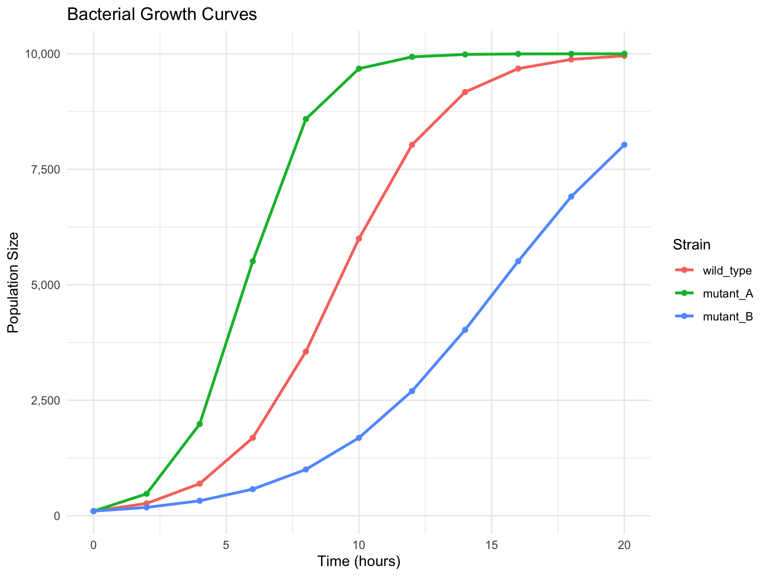
15.8 A Worked Example: Normalizing Gene Counts
The examples so far have been small on purpose. Here is a function of the kind you will actually write, built up in the way functions get built in practice: first as a few lines that work once, then as something reusable. The raw read counts in the stickleback data (Section 1.5) are not directly comparable between fish, because some libraries were sequenced more deeply than others. The usual first step is to scale each fish’s counts to counts per million (CPM), dividing by that fish’s total and multiplying by a million, and often to take a logarithm afterwards so that a handful of very highly expressed genes do not dominate every plot.
Written once, for one column, that is a single line: stickle$Gene1 / rowSums(stickle[, 5:604]) * 1e6. Written for every gene it becomes a loop, and written for the next dataset it becomes a copy of the loop with the column numbers changed by hand, which is exactly the moment Section 15.1 warned about. The function below does the job for any data frame whose gene columns can be named.
library(tidyverse)

normalize_cpm <- function(counts, gene_cols, log = TRUE, pseudocount = 1) {
  # counts:      a data frame with one row per sample
  # gene_cols:   a tidyselect specification of the count columns, e.g. starts_with("Gene")
  # log:         if TRUE, return log2(CPM + pseudocount); if FALSE, return CPM
  # pseudocount: added before the log so that zero counts stay finite
  gene_mat <- counts |> select({{ gene_cols }}) |> as.matrix()
  if (!is.numeric(gene_mat)) stop("The selected gene columns must all be numeric.")
  if (any(gene_mat < 0, na.rm = TRUE)) stop("Counts cannot be negative.")
  library_size <- rowSums(gene_mat, na.rm = TRUE)
  cpm <- gene_mat / library_size * 1e6
  if (log) cpm <- log2(cpm + pseudocount)
  counts |>
    select(-{{ gene_cols }}) |>
    bind_cols(as_tibble(cpm))
}
Several of the chapter’s ideas are at work in these fifteen lines. The arguments have defaults (Section 15.3.3), so the common call is short and the unusual one is still possible. The input checks at the top (Section 15.9.3) fail immediately, with a message that says what went wrong, rather than producing a plausible-looking matrix of nonsense several steps later. The double-brace { gene_cols } is the tidyverse’s way of letting a function accept a column specification such as starts_with("Gene") and pass it on to select(); it is the one piece of syntax here that is specific to writing functions around dplyr, and it is worth recognizing because you will see it in other people’s code. And the function returns a data frame of the same shape it was given, with the sample metadata untouched and the count columns replaced, so it drops straight into a pipeline.
| Individual | Genotype | Microbiota | Geno&Micro | Gene1 | Gene2 | Gene3 |
|---|---|---|---|---|---|---|
| AC1 | A | conventional | convA | 6.372507 | 6.280558 | 8.508702 |
| AC2 | A | conventional | convA | 5.201244 | 4.985373 | 8.527971 |
| AC3 | A | conventional | convA | 5.775734 | 5.609096 | 7.049595 |
| AC4 | A | conventional | convA | 5.415360 | 6.566381 | 6.306388 |
# The raw counts and the normalized values tell different stories about library depth
tibble(raw_total = rowSums(select(stickle, starts_with("Gene"))),
       cpm_total = rowSums(2^select(stickle_cpm, starts_with("Gene")) - 1)) |>
  summary()
#>    raw_total        cpm_total
#>  Min.   :125986   Min.   :1e+06
#>  1st Qu.:190894   1st Qu.:1e+06
#>  Median :204544   Median :1e+06
#>  Mean   :284009   Mean   :1e+06
#>  3rd Qu.:371757   3rd Qu.:1e+06
#>  Max.   :582646   Max.   :1e+06
After normalization every fish’s counts sum to (almost exactly) one million, which is the point: differences between fish now reflect biology rather than how much sequencing each one received. Applying the same function to a second dataset, or with log = FALSE, or with a different pseudocount, is now a one-line change instead of a search-and-replace.
NoteWhen to promote code into a function
A useful rule of thumb is the second copy. The first time you write a block of code, write it inline and get it working. The moment you find yourself copying it, stop and turn it into a function, giving the things that differ between the copies names as arguments. Two copies are a smell; three are a bug waiting to happen, because you will fix one and forget the others.
TipTesting a function you just wrote
Check a new function on an input where you already know the answer before trusting it on real data. A two-row, three-gene data frame made with tibble() is enough to confirm by hand that the rows sum to a million and that log = FALSE returns raw CPM. Keep that check in your script as a comment or a tiny stopifnot(); it costs nothing and catches the day someone changes the function.
15.9 Best Practices for Writing Functions
1. Use Descriptive Names
2. Document Your Functions
Add comments explaining what the function does, its arguments, and return value:
# Calculate the melting temperature of a DNA primer
#
# Uses the Wallace rule for short oligonucleotides (<14 bp)
# or the nearest-neighbor method for longer sequences
#
# Arguments:
#   sequence: DNA sequence (string of A, T, G, C)
#   method: "wallace" or "nearest_neighbor"
#
# Returns:
#   Melting temperature in degrees Celsius

calculate_tm = function(sequence, method = "wallace") {
  seq_upper = toupper(sequence)
  length = nchar(seq_upper)

  a_count = str_count(seq_upper, "A")
  t_count = str_count(seq_upper, "T")
  g_count = str_count(seq_upper, "G")
  c_count = str_count(seq_upper, "C")

  if (method == "wallace" || length < 14) {
    # Wallace rule: Tm = 2(A+T) + 4(G+C)
    tm = 2 * (a_count + t_count) + 4 * (g_count + c_count)
  } else {
    # Simplified nearest-neighbor approximation
    tm = 64.9 + 41 * (g_count + c_count - 16.4) / length
  }

  return(tm)
}

calculate_tm("ATGCGATCGATCG")
#> [1] 40
3. Validate Inputs
Check that inputs are valid before processing:
gc_content_safe = function(sequence) {
  # Check input type
  if (!is.character(sequence)) {
    stop("Sequence must be a character string")
  }

  # Check for valid DNA characters
  seq_upper = toupper(sequence)
  invalid_chars = str_remove_all(seq_upper, "[ATGCN]")
  if (nchar(invalid_chars) > 0) {
    warning(paste("Invalid characters removed:", invalid_chars))
  }

  gc_count = str_count(seq_upper, "[GC]")
  total_bases = str_count(seq_upper, "[ATGC]")

  if (total_bases == 0) {
    stop("No valid DNA bases found in sequence")
  }

  return(gc_count / total_bases)
}

gc_content_safe("ATGCGATCG")     # Works fine
#> [1] 0.5555556
gc_content_safe("ATGCXYZGATCG")  # Warning about invalid characters
#> [1] 0.5555556
4. Keep Functions Focused
Each function should do one thing well. Break complex operations into smaller functions:
# Instead of one giant function, break it up:

# Step 1: Clean the sequence
clean_sequence = function(seq) {
  seq %>%
    toupper() %>%
    str_remove_all("[^ATGC]")
}

# Step 2: Calculate base composition
base_composition = function(seq) {
  tibble(
    A = str_count(seq, "A"),
    T = str_count(seq, "T"),
    G = str_count(seq, "G"),
    C = str_count(seq, "C")
  )
}

# Step 3: Derive statistics
sequence_stats = function(composition) {
  total = sum(composition)
  composition %>%
    mutate(
      total = total,
      gc_content = (G + C) / total,
      at_content = (A + T) / total
    )
}

# Combine them in a pipeline
"atgcGATCgatcgNNNN" %>%
  clean_sequence() %>%
  base_composition() %>%
sequence_stats()| A | T | G | C | total | gc_content | at_content |
|---|---|---|---|---|---|---|
| 3 | 3 | 4 | 3 | 13 | 0.5384615 | 0.4615385 |
15.10 Summary
Writing functions is a fundamental programming skill that will dramatically improve your data analysis workflows:
-
Basic syntax:
function_name = function(args) { body; return(value) } -
Return values: Use explicit
return()statements; return lists or data frames for multiple values - Default arguments: Provide sensible defaults for commonly-used parameter values
- Lexical scoping: Functions operate in their own environment, keeping your global environment clean
-
Control flow: Use
if/elseandcase_when()to handle different conditions -
Functional programming: Prefer
lapply()/map()over for loops for iteration -
Multiple inputs: Use
pmap()or data frame inputs for complex parameter combinations
Chapter 21 will show you how to run functions in parallel, catch errors gracefully (Section 21.7), and cache results for expensive computations (Section 21.8).
Tip
For quick reference on R function syntax and functional programming tools like lapply() and purrr, see Appendix E.
Additional Reading
To deepen your understanding of functions and functional programming in R:
- R for Data Science: Functions (Wickham et al., 2023) — Excellent introduction to writing functions
- Advanced R: Functions by Hadley Wickham — Deep dive into function mechanics
- purrr Documentation — Complete guide to functional programming with purrr
- R for Data Science: Iteration — More on map functions and iteration
For advanced function development:
- Advanced R: Functional Programming — Closures, function factories, and more
- R Packages by Wickham and Bryan — When you’re ready to package your functions
Exercises
TipPractice Exercises
Exercise 1: Basic Function
Write a function called count_codons() that takes a DNA sequence and returns the number of complete codons (groups of 3 nucleotides). For example, “ATGCGA” has 2 complete codons.
Exercise 2: Function with Multiple Returns
Write a function analyze_sequence() that takes a DNA sequence and returns a data frame with: - The sequence length - GC content - Number of each base (A, T, G, C) - Whether it starts with a start codon (ATG) - Whether it ends with a stop codon (TAA, TAG, or TGA)
Exercise 3: Control Flow
Write a function translate_codon() that takes a three-letter codon and returns the corresponding amino acid (use a simplified table with just 5-10 codons). Include error handling for invalid inputs.
Exercise 4: Iteration
You have a vector of 10 DNA sequences. Use map_df() to apply your analyze_sequence() function from Exercise 2 to all of them and combine the results into a single data frame.
Exercise 5: Multiple Inputs
Write a function dilution_series() that takes an initial concentration and dilution factor, then returns a data frame showing the concentration at each step for a specified number of dilutions. Use pmap() to apply this to multiple starting conditions.
Exercise 6: Refactoring
Take the following for loop and rewrite it using functional programming: