16 Reproducible Documents with Quarto
After completing this chapter, you will be able to:
- Explain the benefits of literate programming for reproducible research
- Create Quarto documents that combine code, text, and results
- Use Markdown syntax for text formatting
- Configure document settings with YAML headers
- Control code execution and output with chunk options
- Include mathematical equations and figures
- Run Python (and mixed R/Python) code in a Quarto document
- Use callouts, tabsets, divs, and cross-references to structure a document
- Cite sources from a BibTeX file
- Render documents to multiple output formats from your IDE (VS Code, Positron, or RStudio) and the command line
16.1 What is Quarto?
Quarto is an open-source scientific publishing system that enables you to create dynamic documents combining narrative text, code, and results (Posit Software, PBC, 2024). It represents the next generation of literate programming tools, building on the legacy of R Markdown (Xie et al., 2018) while extending support to multiple programming languages including R, Python, Julia, and Observable JavaScript.
The name “Quarto” comes from the Latin word for a quarter sheet of paper folded twice to create an eight-page booklet—an evocative reference to the history of publishing and scholarly communication. Just as the quarto format revolutionized book publishing in the 16th century, the Quarto system is revolutionizing how scientists share their work.
Quarto documents are plain text files with the .qmd extension that can be rendered to:
- HTML documents and websites
- PDF documents
- Microsoft Word documents
- Presentations (PowerPoint, reveal.js)
- Books (like this one!)
- Interactive dashboards
Why Use Quarto?
Quarto solves fundamental problems in scientific communication:
- Reproducibility
- Your analysis and its documentation live together. Anyone can re-run your code and verify your results.
- Efficiency
- No more copying and pasting results between applications. Update your data, re-render, and all figures and statistics update automatically.
- Transparency
- Readers can see exactly how results were generated. The code is the methods section.
- Collaboration
- Plain text files work seamlessly with version control systems like Git (Chapter 19).
- Flexibility
- Write once, render to multiple formats. The same document can produce a lab report, a presentation, and a web page.
This entire textbook was written in Quarto! You can see the source files in the repository.
The Literate Programming Philosophy
Quarto is built on the concept of literate programming, introduced by Donald Knuth in 1984 (Knuth, 1984). The idea is revolutionary yet simple: instead of writing code with occasional comments, write a human-readable document that happens to contain executable code. As Knuth wrote:
“Let us change our traditional attitude to the construction of programs: Instead of imagining that our main task is to instruct a computer what to do, let us concentrate rather on explaining to human beings what we want a computer to do.”
In practice, this means your analysis scripts become documents that tell a story. The code is woven together with explanations of why you’re doing each step, what you expect to find, and how the results should be interpreted. When you share this document, readers understand not just the mechanical steps, but the reasoning behind each analytical choice.
This approach has profound implications for science:
Your methods become self-documenting. No more separate “methods” documents that drift out of sync with your actual code.
Errors become visible. When code and narrative live together, inconsistencies between what you say you’re doing and what you’re actually doing become obvious.
Learning accelerates. Well-documented analyses serve as tutorials for others (and for your future self) who want to learn your techniques.
Reproducibility becomes the default. Rendering re-runs everything from raw data to final figures, so “can we regenerate this?” stops being a scramble before submission and becomes something that happens every time you press render.
Funders increasingly require that research outputs be FAIR — Findable, Accessible, Interoperable, and Reusable (Wilkinson et al., 2016) — and a literate document delivers each letter in practice. Plain-text .qmd sources and tidy data tables are open formats that every tool can read (interoperable); the methods travel inside the document instead of drifting in a separate file (reusable); and the whole bundle — source, data, and environment — can be deposited in a public repository with a persistent identifier (findable and accessible; Chapter 19). Appendix C works through the principles and a minimal FAIR checklist; Chapter 1 describes the funding policies behind them.
16.2 Markdown: The Foundation
Markdown is a lightweight markup language that lets you add formatting to plain text. Created by John Gruber in 2004, it’s designed to be readable in its raw form while rendering to beautifully formatted documents.
Why Markdown?
Markdown’s appeal lies in its simplicity—there are no complex menus or formatting palettes to learn. You write plain text with a few special characters, and the formatting appears when the document renders. This simplicity makes Markdown incredibly portable: your files work on any computer, in any text editor, without special software. Because Markdown files are plain text, they’re also future-proof—unlike proprietary formats that may become obsolete, text files will always be readable. Finally, plain text is version-control friendly: Git can track every change you make, showing exactly what was added, removed, or modified between versions.
Positron, RStudio, and VS Code can each show a Markdown or Quarto file in two ways: source mode, the raw text exactly as it is stored, and a visual editor that renders headings, bold, and tables as you type, like a lightweight word processor (look for the toggle at the top right of the editor). Both edit the same plain-text file, so nothing is lost by switching back and forth. Learn source mode first—it is what this chapter teaches, what Git shows when files change, and what you will see in everyone else’s files—and reach for the visual editor where it shines: editing tables and inserting citations.
Basic Text Formatting
Renders as:
italic text or italic text
bold text or bold text
bold and italic or bold and italic
strikethrough text
inline code
Headers
Create hierarchical structure with headers:
In Quarto books, each chapter typically starts with a single # header, with subsequent sections using ## and ###.
Lists
Unordered lists use asterisks, hyphens, or plus signs:
- Item one
- Item two
  - Nested item (indent with 2 spaces)
  - Another nested item
- Item three
Ordered lists use numbers:
- First step
- Second step
- Third step
- Sub-step
- Another sub-step
Task lists add a checkbox to each item (rendered in HTML output):
Links and Images
A bare URL in angle brackets becomes a clickable link with the URL as its text.
Blockquotes
This is a blockquote. Use it for quotations or to highlight important text.
Multiple paragraphs work too.
Code Blocks
For displaying code without execution, use fenced code blocks with language specification:
Tables
Create tables with pipes and hyphens (the result is Table 16.1):
| Column 1 | Column 2 | Column 3 |
|---|---|---|
| Left | Center | Right |
| aligned | aligned | aligned |
The colons indicate alignment: :--- left, :---: center, ---: right.
Tables produced by code. Most tables in a report come from a code chunk rather than being typed by hand. Give the chunk a label starting with tbl- and a tbl-cap, and the table becomes numbered and cross-referenceable exactly like a hand-written one:
knitr::kable() is the simplest R option; the gt package (used throughout Chapter 14) produces publication-quality tables from the same pipeline.
Horizontal Rules
Create a horizontal divider with three or more hyphens, asterisks, or underscores:
Footnotes
Add footnotes for additional context without interrupting the flow:
This is a statement that needs a citation.1
Definition Lists
Define terms with a colon-based syntax:
- Term 1
- Definition of the first term.
- Term 2
- Definition of the second term.
- You can have multiple definitions.
Line Breaks and Paragraphs
In Markdown, a single line break is ignored—you need a blank line to create a new paragraph. To force a line break without a new paragraph, end the line with two spaces or use <br>.
Table 16.2 collects the syntax introduced above.
| Format | Syntax | Result |
|---|---|---|
| Bold | **text** |
text |
| Italic | *text* |
text |
| Code | `code` |
code |
| Link | [text](url) |
text |
| Strikethrough | ~~text~~ |
|
| Subscript | H~2~O |
H2O |
| Superscript | 10^2^ |
102 |
16.3 Quarto Document Structure
A Quarto document has three main parts:
- YAML Header: Document metadata and settings
- Markdown Content: Text and formatting
- Code Chunks: Executable code blocks
YAML Header
The YAML header appears at the top of the document, enclosed by triple dashes:
YAML stands for “YAML Ain’t Markup Language” (a recursive acronym). It uses key-value pairs with consistent indentation.
Common YAML Options
| Option | Description |
|---|---|
title |
Document title |
author |
Author name(s) |
date |
Publication date (today for current date, or "2025-01-15") |
format |
Output format(s) |
toc |
Include table of contents |
toc-depth |
How many header levels in TOC |
number-sections |
Number the section headings |
code-fold |
Collapse code by default |
execute |
Global code execution options (echo, warning, message, …) |
bibliography |
BibTeX file for citations (Section 16.10) |
YAML is indentation-sensitive: nested options must be indented with spaces (never tabs), and a colon must be followed by a space. An error such as “YAML parse exception” almost always means a mis-indented line or a missing quote around a value that contains a colon.
16.4 Code Chunks
Code chunks are the heart of Quarto’s power—they let you embed executable code directly in your document.
Basic Syntax
In Quarto, code chunks use this syntax:
Chunk Options
Control chunk behavior with special comments starting with #|:
Essential Chunk Options
The options you will use most are listed in Table 16.4.
| Option | Description | Default |
|---|---|---|
echo |
Show code in output | true |
eval |
Execute the code | true |
include |
Include chunk in output | true |
output |
Show results | true |
warning |
Show warnings | true |
message |
Show messages | true |
error |
Continue on error | false |
cache |
Cache results | false |
label |
Name the chunk (and its cross-reference id) | none |
fig-cap / tbl-cap
|
Caption a figure / table | none |
code-fold |
Collapse the code behind a toggle | false |
echo: fenced |
Show the chunk with its fence and options (for teaching) | — |
Set defaults for every chunk in the YAML execute: block (Table 16.3) and override per chunk only where needed. A hidden setup chunk at the top of a document is typically #| include: false.
Controlling Output
#>     Min.  1st Qu.   Median     Mean  3rd Qu.     Max.
#> -2.58685 -0.82420  0.06269 -0.05193  0.60584  2.49475
Hide code, show results (great for final reports):
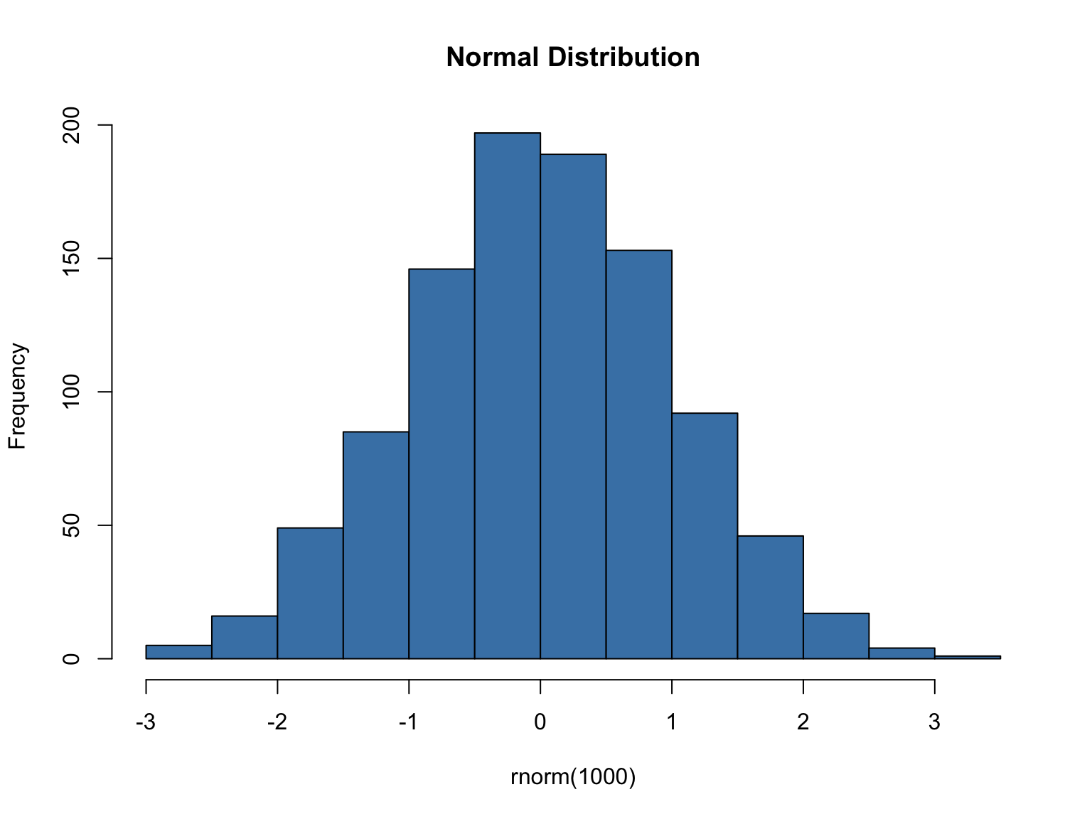
Show code, hide results (for teaching):
Figure Options
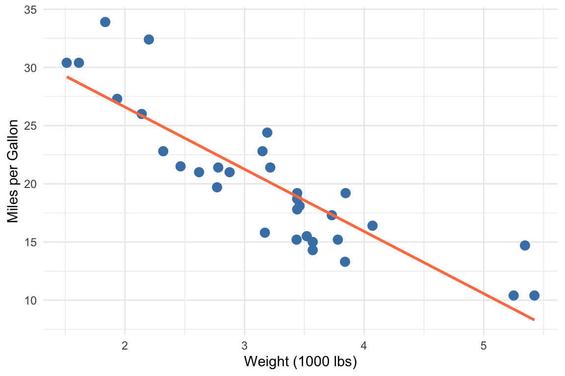
Control figure appearance with the options in Table 16.5; Figure 16.2 below is produced by such a chunk:
| Option | Description |
|---|---|
fig-cap |
Figure caption |
fig-width |
Width in inches |
fig-height |
Height in inches |
fig-align |
Alignment: left, center, right |
out-width |
Output width (e.g., “80%”) |
fig-dpi |
Resolution of raster output (e.g., 300 for print) |
fig-format |
Format: png, svg, pdf |
fig-subcap |
List of sub-captions for a chunk that draws several plots |
layout-ncol |
Number of columns to arrange multiple plots in |
Subfigures. A chunk that produces more than one plot can label each with fig-subcap and arrange them with layout-ncol; the panels are referenced as @fig-label-1, @fig-label-2, and so on:
Inline Code
A computed value does not need a whole chunk. An inline expression—a short piece of code inside a sentence—is evaluated at render time and its result typeset in place:
This is the mechanism behind the promise that numbers in your prose can never disagree with your data: “We measured 80 fish” is computed, not typed, so re-rendering after the data change updates the sentence along with every figure (Section 16.18 shows it in action). Older knitr documents write the R form without the braces—the expression follows r directly after the opening backtick; both forms work in Quarto. Keep inline expressions to a single short call—compute anything substantial in a chunk, store it in a variable, and reference the variable inline.
16.5 Python in Quarto
Everything above works unchanged for Python: replace {r} with {python} and the chunk runs when the document renders. The mechanics differ in one respect. R chunks are executed by the knitr engine, which ships with R; Python chunks are executed by the Jupyter engine, so you need a Python environment with Jupyter installed (Section 12.3):
Quarto chooses the engine from the first chunk it sees, or you can state it in the YAML header:
A {python} chunk accepts the same #| options as an R chunk (echo, eval, fig-cap, label, and so on), and a matplotlib or seaborn figure produced in a chunk labelled fig-... with a fig-cap becomes a cross-referenceable figure exactly as a ggplot does.
Mixing R and Python in one document. A document can use only one engine, but the knitr engine can run Python chunks through the reticulate R package: install.packages("reticulate"), then {python} chunks in an otherwise-R document execute in a Python session, and objects pass between languages as py$name (in R) and r.name (in Python). This is the route to take when most of a document is R and a step or two is Python.
Jupyter notebooks. Quarto also renders .ipynb files directly, so an existing notebook needs no conversion:
By default Quarto uses the outputs already stored in the notebook; add --execute to re-run it during rendering. Section 2.9 compares the two formats, and Chapter 12 introduces the Python language itself.
16.6 Mathematical Equations
Quarto supports LaTeX math notation for equations; Chapter 17 covers the notation in depth, and Appendix G is a symbol reference.
Inline Math
Use single dollar signs for inline equations:
The mean is calculated as \(\bar{x} = \frac{1}{n}\sum_{i=1}^{n} x_i\).
Display Math
Use double dollar signs for centered equations:
\[ \sigma^2 = \frac{1}{n-1}\sum_{i=1}^{n}(x_i - \bar{x})^2 \]
Common Math Notation
Table 16.6 lists the constructs you will need most often.
| Symbol | Code | Result |
|---|---|---|
| Greek letters | $\alpha, \beta, \gamma$ |
\(\alpha, \beta, \gamma\) |
| Subscript | $x_1, x_{12}$ |
\(x_1, x_{12}\) |
| Superscript | $x^2, x^{10}$ |
\(x^2, x^{10}\) |
| Fraction | $\frac{a}{b}$ |
\(\frac{a}{b}\) |
| Square root | $\sqrt{x}$ |
\(\sqrt{x}\) |
| Sum | $\sum_{i=1}^{n}$ |
\(\sum_{i=1}^{n}\) |
| Product | $\prod_{i=1}^{n}$ |
\(\prod_{i=1}^{n}\) |
| Integral | $\int_0^1 f(x)dx$ |
\(\int_0^1 f(x)dx\) |
Example: Statistical Formulas
The probability density function of a normal distribution:
\[ f(x) = \frac{1}{\sigma\sqrt{2\pi}} e^{-\frac{1}{2}\left(\frac{x-\mu}{\sigma}\right)^2} \]
A regression equation:
\[ Y_i = \beta_0 + \beta_1 X_{1i} + \beta_2 X_{2i} + \epsilon_i \]
16.7 Callout Blocks
Quarto provides special callout blocks for highlighting information:
::: {.callout-note}
This is a note callout for additional information.
:::

::: {.callout-warning}
This warns readers about potential issues.
:::

::: {.callout-important}
This highlights critical information.
:::

::: {.callout-tip}
This provides helpful tips.
:::

::: {.callout-caution}
This urges caution.
:::

::: {.callout-tip title="A custom title"}
Add `title="..."` for your own heading.
:::

::: {.callout-note collapse="true"}
Add `collapse="true"` and the box starts folded; click to open.
:::This is a note callout for additional information.
This warns readers about potential issues.
This provides helpful tips.
This one starts folded. Collapsed callouts are handy for optional detail or exercise answers.
The five types differ only in icon and color; pick by meaning (Table 16.7).
| Type | Color | Use for |
|---|---|---|
note |
Blue | Supplementary information |
tip |
Green | Helpful suggestions and shortcuts |
warning |
Orange | Potential problems or common mistakes |
important |
Red | Information the reader must not miss |
caution |
Red | Dangerous or irreversible operations |
A callout is a fenced div: a line of three or more colons with the class in braces, the content, and a closing line of colons. The opening and closing fences must each sit on their own line with a blank line around the block, or the div will not close and the rest of the page renders inside the box.
16.8 Tabsets, Divs, and Spans
The same ::: fence syntax gives you several other structures.
Tabsets present alternatives (R vs. Python, source vs. output) in tabs. Every heading inside the div becomes a tab:
Layout divs arrange their children. {layout-ncol=2} places two figures side by side; {.column-margin} pushes content into the margin; {.column-page} lets a wide table use the full page width:
Generic attributes in braces can follow any div, heading, image, or code block: an id (#name), classes (.name), and key-value pairs. This is how headings get cross-reference ids and how images get sizes and alt text:
Spans apply attributes to a run of inline text with [text]{...}:
Nested divs need more colons on the outside (:::: around :::) so that Quarto can tell which fence closes which block.
16.9 Cross-References
Reference figures, tables, and sections:
Figures and Tables
See Figure 16.2 for the scatter plot. The options are listed in Table 16.4.
Sections
As discussed in Chapter 16, Quarto enables reproducible documents.
The label prefix determines the reference type (Table 16.8). A code chunk becomes a referenceable figure when its label starts with fig- and it has a fig-cap; Markdown tables take their id from the caption line : Caption {#tbl-id}. Quarto numbers everything automatically, so inserting a figure renumbers the rest.
| Type | Prefix | Where the id goes | Reference |
|---|---|---|---|
| Figure | fig- |
#| label: fig-name or {#fig-name}
|
@fig-name |
| Subfigure | fig- |
fig-subcap panels of fig-name
|
@fig-name-1 |
| Table | tbl- |
#| label: tbl-name or : Caption {#tbl-name}
|
@tbl-name |
| Section | sec- |
## Heading {#sec-name} |
@sec-name |
| Equation | eq- |
$$ ... $$ {#eq-name} |
@eq-name |
| Code listing | lst- |
#| label: lst-name with lst-cap
|
@lst-name |
Quarto also recognises thm-, lem-, def-, exm-, and exr- for theorem-style blocks (::: {#thm-clt}). Capitalize the prefix (@Fig-name) to begin a sentence with “Figure” rather than “fig.”
Equations
The label must sit on the same line as the closing $$, separated by a space. Only labelled equations are numbered. Section 17.13 shows how to align a multi-line derivation under one number.
16.10 Citations
Quarto handles references the same way it handles cross-references: each source has a key, and you cite the key with @. The keys live in a BibTeX file (.bib), a plain-text database in which each entry looks like this:
Name the file in the YAML header, then cite by key:
---
title: "Report"
bibliography: references.bib
---

Knuth introduced literate programming [@knuth1984literate].
@knuth1984literate argued that programs should be written for people.
Several authors agree [@knuth1984literate; @xie2018r].
A page reference [@knuth1984literate, p. 99] or a prefix [see @knuth1984literate].
Bracketed citations render in parentheses, “(Knuth 1984)”; a bare @key renders in the running text, “Knuth (1984)”. Quarto compiles a reference list at the end of the document automatically, or wherever you place a ::: {#refs} div. The default style is Chicago author-date; add csl: apa.csl (any style file from the CSL repository) to change it.
Reference managers such as Zotero export BibTeX directly, and Google Scholar’s “Cite” button offers a BibTeX entry for any paper. Keep one references.bib per project and let it grow.
16.11 Rendering Documents
Rendering is the step that turns the plain-text source into a finished document. Quarto reads the .qmd file, runs every code chunk through R or Python (via knitr or Jupyter), weaves the results into the Markdown, and hands the whole thing to Pandoc, which produces the output format you asked for (Figure 16.3). Because the code runs every time, the numbers, tables, and figures in the output can never drift away from the code that produced them.
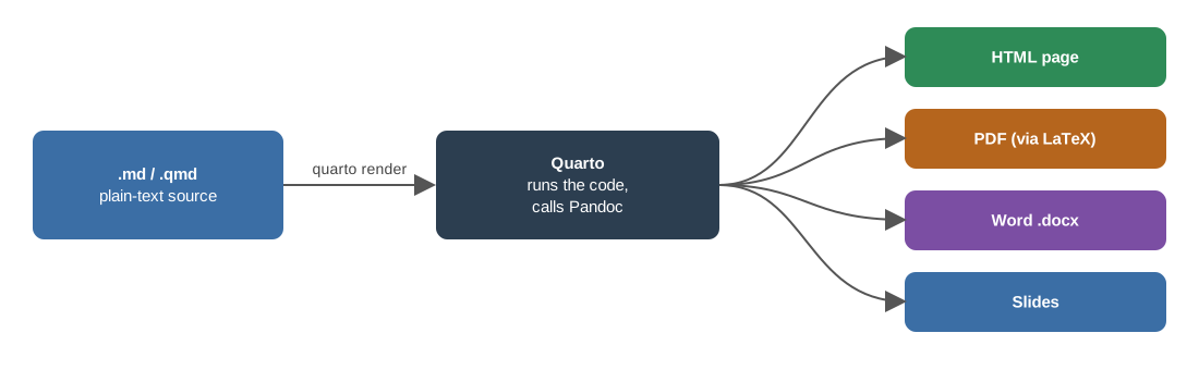
.qmd file, run through Quarto, becomes an HTML page, a PDF (via LaTeX), a Word document, or a slide deck.
From VS Code, Positron, or RStudio
- Click the Preview button (VS Code and Positron, Quarto extension) or the Render button (RStudio), or
- Use the keyboard shortcut, the same in all three:
Ctrl+Shift+K(Windows/Linux) orCmd+Shift+K(Mac)
While writing, Ctrl+Alt+I / Cmd+Option+I inserts a new code chunk and Ctrl+Shift+Enter / Cmd+Shift+Enter runs the current chunk without rendering the whole document (more in Appendix A).
Rendering starts a fresh session and runs the document top to bottom, so nothing from your interactive session—packages you loaded by hand, objects you created at the console, a chunk you ran and then deleted—exists during the render. This is the most common Quarto surprise: a chunk that “just worked” interactively fails with object not found or could not find function when you render. It is a feature, not a bug: a successful render is proof that the document is self-contained and your analysis actually reproducible. The habits that follow from it: load every package in the document’s first chunk, create everything the document uses inside the document, and render early and often rather than once at the deadline, so problems surface one at a time.
From Command Line
Live Preview
For interactive editing:
This opens a browser window that automatically updates as you edit. --port 8080 fixes the port and --no-browser prints the URL instead of opening a window (useful on a remote machine).
The Quarto Command Line
The quarto program has a handful of subcommands you will use regularly (Table 16.9).
| Command | What it does |
|---|---|
quarto render file.qmd |
Render to the document’s default format |
quarto render file.qmd --to pdf |
Render to one format (html, pdf, docx, revealjs, …) |
quarto render file.qmd --to all |
Render every format listed in the YAML |
quarto render file.qmd --output out.html |
Choose the output file name |
quarto render file.qmd -P n:100 |
Set a document parameter (params: in YAML) |
quarto render |
Render the whole project (_quarto.yml) |
quarto preview file.qmd |
Live preview that re-renders on save |
quarto create project |
Scaffold a new project, website, or book |
quarto check |
Verify the installation (R, Python/Jupyter, LaTeX) |
quarto install tinytex |
Install a minimal LaTeX so PDF rendering works |
quarto publish gh-pages |
Publish the rendered site (see Section 19.11) |
quarto --version |
Print the installed version |
16.12 Multiple Output Formats
Render to multiple formats from one source:
Then render all formats:
Without --to all, quarto render produces only the first format listed. Each format accepts its own options, nested under its name.
HTML Options
HTML is the richest target: it supports folding code, tabsets, interactive figures, and a floating table of contents.
| Option | Description | Values |
|---|---|---|
toc-location |
Where the TOC sits |
left, right, body
|
code-fold |
Collapse code behind a toggle |
true, false, show
|
code-tools |
Menu to view/copy the full source |
true, false
|
theme |
Bootswatch visual theme |
default, cosmo, flatly, darkly, … |
embed-resources |
Bundle images, CSS, and JS into one .html file |
true, false
|
embed-resources: true is the option to remember when you email a report: without it the HTML file depends on a folder of supporting files that must travel with it.
PDF Options
PDF output passes through LaTeX (Chapter 17), so a LaTeX installation is required (quarto install tinytex provides a small one).
| Option | Description | Values |
|---|---|---|
documentclass |
LaTeX document class |
article, report, book
|
geometry |
Page size and margins |
margin=1in, letterpaper, … |
fontsize |
Body text size |
10pt, 11pt, 12pt
|
colorlinks |
Colored rather than boxed hyperlinks |
true, false
|
keep-tex |
Keep the intermediate .tex file for debugging |
true, false
|
Word Options
Word output is the format collaborators without Quarto can edit. A reference document supplies the styles (fonts, heading sizes, margins) that the generated .docx inherits, so a journal’s or lab’s template can be applied without touching the source:
Run quarto pandoc -o custom-reference.docx --print-default-data-file reference.docx to obtain a starting template, edit its styles in Word, and point reference-doc at the result.
16.13 Presentations with RevealJS
Set format: revealjs and the same machinery — Markdown, chunks, callouts, math, cross-references — produces a browser-based slide deck instead of a page. The course’s lecture slides are built exactly this way.
---
title: "My Research in Six Slides"
author: "Your Name"
format:
  revealjs:
    theme: default        # simple, serif, moon, solarized, dark, ...
    slide-number: true
    footer: "Lab meeting - November 2026"
    incremental: false    # true = every list reveals point by point
    chalkboard: true      # draw on your slides while presenting
---
The structure rules are simple: every level-2 heading (##) starts a new slide, and a level-1 heading (#) makes a section-divider slide. Beyond that, a handful of presentation-specific tools cover most of what a scientific talk needs:
Revealing content stepwise. Wrap a list in ::: {.incremental} to step through it with the arrow key, or put three spaced dots on their own line (. . .) to pause anything mid-slide. Any block with the .fragment class appears on a keypress.
Columns. A :::: columns div containing two ::: {.column width="45%"} divs puts text beside a figure, or two figures side by side — the most common slide layout in a research talk.
Executed code on slides. Chunks run at render time exactly as in documents, so a figure on a slide is regenerated from data on every render. Two chunk options earn their keep in decks: output-location: slide puts a chunk’s figure on its own slide, and code-line-numbers: "1-2|4|6" highlights groups of lines one keypress at a time — ideal for walking an audience through code.
Speaker notes. A ::: {.notes} div at the end of a slide is invisible to the audience; press S while presenting for the speaker view with notes and a timer. Press O for a zoomed-out overview of the whole deck, F for fullscreen.
The same source also renders to PowerPoint (quarto render deck.qmd --to pptx) or LaTeX Beamer (--to beamer) when a conference insists; simple layouts survive the trip best.
The Week 7 example example_slides.qmd on the course Example Files page demonstrates all of the above in twelve compact slides. Render it, press S and O to try the presenter tools, then change the theme in the YAML and render again.
16.14 Scholarly Manuscripts
A journal manuscript is a Quarto document with three extra ingredients: scholarly front matter, a citation style, and the discipline of echo: false.
Scholarly front matter. Authors can be structured objects rather than plain strings, carrying affiliations, ORCID iDs, and the corresponding-author flag; abstract and keywords complete the title page:
---
title: "Matrix stiffness tunes gene expression in the gut"
author:
  - name: Avery J. Rivers
    orcid: 0000-0002-1825-0097
    corresponding: true
    email: arivers@uoregon.edu
    affiliations:
      - ref: kc
affiliations:
  - id: kc
    name: University of Oregon
    department: Knight Campus for Accelerating Scientific Impact
abstract: |
  One paragraph, 150-200 words, no citations.
keywords: [extracellular matrix, mechanotransduction]
---
Results, never code. Set echo: false document-wide (under execute: in the YAML): readers of a manuscript see figures, tables, and numbers — all still regenerated from the embedded code on every render, with inline code keeping the values in your sentences honest (Section 16.4.6).
Citations in the journal’s style. Name a .bib file and a CSL style file in the YAML (Section 16.10) and every citation and the reference list are formatted for that journal — nature.csl gives numbered superscripts, apa.csl gives author-year, and the CSL repository has a file for essentially every journal. Changing journals means changing one line, not re-typing references.
Everything numbered and cross-referenced. Figures, tables, display equations ($$ ... $$ {#eq-...}), and sections all take labels and @-references (Section 16.9), so “Equation 2” and “Figure 3” renumber themselves when reviewers ask you to reorder.
Two PDF-specific notes. First, journals often want line numbers on submissions — add \usepackage{lineno} and \linenumbers through include-in-header. Second, Quarto’s default PDF template prints author names but silently drops affiliations; the fix is either a small template-partials file that rebuilds the title block, or a ready-made journal format extension (quarto add quarto-journals/nature and friends — see the journal formats gallery).
The Week 7 example example_manuscript.qmd on the course Example Files page is a complete Science/Nature-style article: scholarly front matter, lorem-ipsum sections, inline and display LaTeX, numbered equations, cross-references everywhere, superscript citations from its companion example_manuscript.bib and nature.csl, and a commented title.tex partial that restores affiliations on the PDF title page. It is the intended skeleton for your term project report — copy it, keep the companion files beside it, and replace the lorem ipsum with your science.
16.15 Project Organization
For multi-document projects (like this book), use a _quarto.yml file:
16.16 Websites
A Quarto website is a project whose pages share a navigation bar: set type: website in _quarto.yml, and every .qmd in the folder becomes a page of the site. This is how the course website — and a typical personal academic site — is built.
Two conveniences do most of the work. About pages: adding an about: block (template trestles, jolla, solana, …) to index.qmd lays out a landing page with your photo, a bio, and link buttons to GitHub, Google Scholar, and email — no HTML required. Live preview: quarto preview run inside the folder serves the site locally and re-renders every time you save, so you edit with the result in view; quarto render writes the finished site into output-dir.
A rendered website is just a folder of HTML — the missing step is hosting, and that is Week 8: push the folder to GitHub and serve it with GitHub Pages (Section 19.11), either from docs/ on the main branch or with quarto publish gh-pages.
The Week 7 example example_website.zip on the course Example Files page is a complete four-page academic site for a fictional graduate student — home/about, research, publications, CV — pre-configured with output-dir: docs for GitHub Pages. Unzip it, run quarto preview inside it, replace Avery’s details with yours, and keep it: it goes live in Week 8.
16.17 Best Practices
Document Structure
- Start with clear objectives: What should readers learn?
- Organize hierarchically: Use headers to create logical sections
- Balance code and narrative: Explain the “why” not just the “what”
-
Use meaningful chunk labels:
#| label: fig-gene-expressionnot#| label: chunk1
Code Quality
- Show relevant code: Hide boilerplate, show analysis
- Comment your code: Explain complex operations
- Use consistent style: Follow a style guide (tidyverse, etc.)
- Set global options: Configure defaults in YAML, override as needed
Reproducibility
- Document your environment: Include package versions
-
Use relative paths: Avoid
/Users/yourname/... - Set a random seed: For reproducible random operations
- Version control: Track your .qmd files with Git (Chapter 19); GitHub Pages can publish the rendered site (Section 19.11)
# Document your R environment
sessionInfo()
#> R version 4.6.0 (2026-04-24)
#> Platform: aarch64-apple-darwin23
#> Running under: macOS 27.0.1
#>
#> Matrix products: default
#> BLAS:   /Library/Frameworks/R.framework/Versions/4.6/Resources/lib/libRblas.0.dylib
#> LAPACK: /Library/Frameworks/R.framework/Versions/4.6/Resources/lib/libRlapack.dylib;  LAPACK version 3.12.1
#>
#> locale:
#> [1] en_US.UTF-8/en_US.UTF-8/en_US.UTF-8/C/en_US.UTF-8/en_US.UTF-8
#>
#> time zone: America/Los_Angeles
#> tzcode source: internal
#>
#> attached base packages:
#> [1] stats     graphics  grDevices utils     datasets  methods   base
#>
#> other attached packages:
#>  [1] gt_1.3.0        lubridate_1.9.5 forcats_1.0.1   stringr_1.6.0
#>  [5] dplyr_1.2.1     purrr_1.2.2     readr_2.2.0     tidyr_1.3.2
#>  [9] tibble_3.3.1    ggplot2_4.0.3   tidyverse_2.0.0
#>
#> loaded via a namespace (and not attached):
#>  [1] Matrix_1.7-5       gtable_0.3.6       jsonlite_2.0.0     compiler_4.6.0
#>  [5] tidyselect_1.2.1   xml2_1.5.2         splines_4.6.0      scales_1.4.0
#>  [9] yaml_2.3.12        fastmap_1.2.0      lattice_0.22-9     R6_2.6.1
#> [13] labeling_0.4.3     generics_0.1.4     knitr_1.51         htmlwidgets_1.6.4
#> [17] pillar_1.11.1      RColorBrewer_1.1-3 tzdb_0.5.0         rlang_1.2.0
#> [21] stringi_1.8.7      xfun_0.58          fs_2.1.0           S7_0.2.2
#> [25] otel_0.2.0         timechange_0.4.0   cli_3.6.6          mgcv_1.9-4
#> [29] withr_3.0.2        magrittr_2.0.5     digest_0.6.39      grid_4.6.0
#> [33] hms_1.1.4          nlme_3.1-169       lifecycle_1.0.5    vctrs_0.7.3
#> [37] evaluate_1.0.5     glue_1.8.1         farver_2.1.2       rmarkdown_2.31
#> [41] tools_4.6.0        pkgconfig_2.0.3    htmltools_0.5.9
16.18 Running Example: The Stickleback Data
This section applies the chapter to the course dataset described in Section 1.5 (80 stickleback, 4 treatment groups, 600 genes). The same steps appear on the Week 7 slides, so the book and the lecture can be read side by side.
Everything the course has done with the stickleback data can live in one Quarto document: the prose, the analysis, the figure, and the numbers quoted in the text, all regenerated on every render. A minimal report looks like this:
---
title: "Genotype and microbiota effects on gut gene expression"
author: "Your Name"
format: html
---

```{r}
#| label: setup
#| message: false
library(tidyverse)
stickle <- read_tsv("data/Stickle_RNAseq.tsv", show_col_types = FALSE)
long <- stickle |> pivot_longer(starts_with("Gene"), names_to = "gene", values_to = "count")
```

We measured `r n_distinct(long$gene)` genes in `r nrow(stickle)` fish
(@fig-gene1).

```{r}
#| label: fig-gene1
#| fig-cap: "Gene1 counts by genotype and microbiota."
ggplot(filter(long, gene == "Gene1"), aes(Genotype, count, fill = Microbiota)) + geom_boxplot()
```
The inline code means the sentence “We measured 600 genes in 80 fish” is computed, not typed, so it can never disagree with the data. The chunk label beginning with fig- makes the figure numbered and cross-referenceable. Add format: pdf to the header, once TinyTeX is installed (Section 2.3.5), and the same file becomes a manuscript-ready PDF; add format: revealjs and it becomes slides.
16.19 Summary
Quarto transforms how we communicate scientific work:
- Markdown provides simple, readable formatting syntax
- YAML headers configure document settings
- Code chunks embed executable, reproducible analysis
-
Python chunks run through Jupyter (or reticulate), and Quarto renders
.ipynbnotebooks directly -
Callouts, tabsets, and divs structure a document with the same
:::fence syntax - Multiple formats serve different audiences from one source
-
Cross-references and citations create professional, navigable documents from
@-keys and a.bibfile -
The same toolkit scales up:
format: revealjsfor talks, scholarly front matter plus a CSL style for journal manuscripts, and website projects for your academic presence on the web
The investment in learning Quarto pays dividends every time you write a report, prepare a presentation, or publish research. Your future self (and your collaborators) will thank you for the reproducibility.
Additional Reading
- Quarto Documentation — Official comprehensive guide
- Quarto Gallery — Examples and templates
- R Markdown Cookbook — Many techniques apply to Quarto
- Markdown Guide — Comprehensive Markdown reference
- Quarto: RevealJS presentations — Every slide feature, with examples
- Quarto: Websites — Site structure, navigation, and about pages
- Quarto: Journal formats — Ready-made article formats for many publishers
Exercises
Exercise 1: First Quarto Document
- Create a new file called
first_report.qmd - Add a YAML header with title, author, and date
- Write a brief introduction using headers, bold, and italic text
- Include a bulleted list of your analysis goals
- Render to HTML
Exercise 2: Code Integration
- Create a document that loads a dataset (use
mtcarsor similar) - Add a code chunk that calculates summary statistics
- Add a code chunk that creates a figure with a caption
- Use chunk options to hide code but show results for one chunk
- Use chunk options to show code but hide results for another
Exercise 3: Mathematical Notation
- Write a document explaining a statistical concept
- Include at least one inline equation
- Include at least one display equation
- Use appropriate callout blocks for tips and warnings
Exercise 4: Multi-Format Output
- Configure your document to render to both HTML and PDF
- Render both versions with
quarto render --to all - Note any differences in how content appears
- Adjust settings to optimize for each format
Exercise 5: Tables, Cross-References, and Citations
- Type a small pipe table by hand and give it a caption with a
{#tbl-...}id - Produce a second table from code (
knitr::kable(head(iris, 5))orpandas) with atbl-label andtbl-cap - Refer to both tables and to one figure from the text with
@ - Create a
references.bibwith two entries, addbibliography:to the YAML, and cite both sources (one in brackets, one in running text) - Render and check that the numbering and reference list are generated automatically
Exercise 6: One Toolkit, Three Outputs
- Download the three Week 7 examples from the course Example Files page — the slide deck, the manuscript with its companion files, and the website zip
- Render
example_slides.qmd, then change thetheme:and add one new slide containing an executed code chunk - In the manuscript, add one reference to the
.bibfile and cite it, add one numbered equation and reference it from the text, and re-render (to PDF with TinyTeX, otherwise to HTML) - Unzip the website, run
quarto previewinside the folder, and replace the fictional student’s name, photo, and research blurbs with your own - Keep the personalized site — it becomes your live GitHub Pages site in Week 8 (Section 19.11)
This is the footnote content.↩︎