After completing this chapter, you will be able to:
Explain the Grammar of Graphics philosophy underlying ggplot2
Distinguish between mapping an aesthetic to a variable and setting it to a constant
Choose a chart type from the types of variables and the question being asked
Create common plot types: scatter plots, histograms, box plots, bar charts
Customize plots with colors, labels, scales, and themes
Use faceting to create multi-panel figures
Apply data visualization best practices, including honest axes and accessible colour
Recognize and avoid common visualization pitfalls
Save figures in the right format and resolution
13.1 Why Visualize Data?
Before diving into the mechanics of creating plots, it’s worth asking: why visualize data at all? Why not just report the numbers?
The answer lies in how our brains process information. The human visual system has evolved over millions of years to detect patterns, spot outliers, and perceive relationships. A well-designed visualization leverages this natural capability, allowing us to understand complex datasets almost instantly.
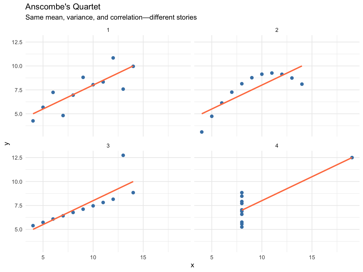
Consider the famous Anscombe’s Quartet(Anscombe, 1973)—four datasets that have nearly identical summary statistics (same mean, variance, and correlation) but tell completely different stories when plotted (Figure 13.1):
# Anscombe's Quartet demonstrationanscombe_long <- anscombe |>pivot_longer(everything(),names_to =c(".value", "set"),names_pattern ="(.)(.)")ggplot(anscombe_long, aes(x = x, y = y)) +geom_point(size =2, color ="steelblue") +geom_smooth(method ="lm", se =FALSE, color ="coral") +facet_wrap(~set, ncol =2) +labs(title ="Anscombe's Quartet",subtitle ="Same mean, variance, and correlation—different stories") +theme_minimal()
Figure 13.1: Anscombe’s Quartet: Four datasets with identical summary statistics but very different patterns
All four datasets have nearly identical statistical summaries, yet they represent fundamentally different phenomena: a linear relationship, a curved relationship, an outlier-driven relationship, and a vertical cluster with one outlier. This example powerfully demonstrates that summary statistics alone can hide important patterns. Visualization reveals what numbers cannot.
ImportantAlways Visualize Your Data
Never trust summary statistics alone. Before running any analysis, plot the data to check its shape, spot outliers, and understand the patterns you are about to model.
13.2 The Grammar of Graphics
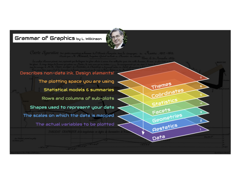
ggplot2 is R’s most popular visualization package (Wickham, 2016), built on Leland Wilkinson’s “Grammar of Graphics”—a framework that describes the fundamental components from which every statistical graphic can be built. Just as grammar provides rules for constructing sentences from words, the grammar of graphics provides rules for constructing visualizations from components: data, aesthetic mappings that connect variables to visual properties, and geometric objects that represent the data, plus scales, statistical transformations, coordinate systems, and facets for finer control.
Seven Components of a Graphic
Every ggplot2 visualization is built from these components (Table 13.1 and Figure 13.2):
Table 13.1: Components of the Grammar of Graphics
Component
Description
Example
Data
The dataset being visualized
mtcars, iris
Aesthetics
Mappings from data to visual properties
x, y, color, size, shape
Geometries
Visual elements representing data
points, lines, bars
Facets
Subplots for data subsets
panels by category
Statistics
Transformations of data
binning, smoothing
Coordinates
The coordinate system
Cartesian, polar
Themes
Non-data visual elements
fonts, backgrounds
Figure 13.2: The Grammar of Graphics framework
13.3 Building a Plot Layer by Layer
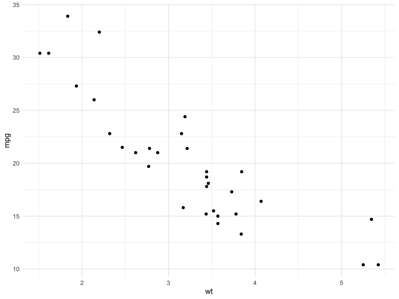
ggplot2 builds plots incrementally using the + operator (Figure 13.3):
# Start with data and aestheticsggplot(data = mtcars, aes(x = wt, y = mpg)) +# Add a geometry layergeom_point()
Figure 13.3: A minimal ggplot2 scatter plot of car weight against fuel efficiency
Let’s break this down:
ggplot() initializes the plot with data
aes() maps variables to visual properties (aesthetics)
One of the most important decisions in visualization is selecting the appropriate chart type for your data and message. Different charts excel at different tasks (Table 13.2):
Table 13.2: Matching questions to chart types
Question
Chart Type
Why
How are values distributed?
Histogram, density plot
Shows shape, center, spread
How do groups compare?
Box plot, bar chart
Side-by-side comparison
How do two variables relate?
Scatter plot
Shows correlation, patterns
How does a value change over time?
Line plot
Connects sequential observations
What is the composition?
Stacked bar, pie chart
Shows parts of a whole
ImportantStart with the Question
Before creating any visualization, ask yourself: “What question am I trying to answer?” The chart type should emerge from the question, not the other way around.
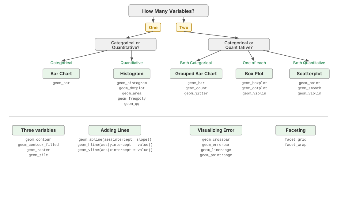
The second input to the decision is the type of each variable you want to show (Section 8.6). Figure 13.4 walks through the choice:
One categorical variable: bar chart of counts
One continuous variable: histogram or density plot
One continuous and one categorical: box plots or violin plots side by side
Two continuous variables: scatter plot, with a line if the x variable is ordered (time)
Two categorical variables: grouped or stacked bar chart, or a heat map of counts
Three or more variables: map the extras to colour, shape, or size, or split them into facets (Section 13.7)
Figure 13.4: A flow chart for choosing a plot type from the number and types of variables to display.
13.5 Essential Geoms
Scatter Plots with geom_point()
Scatter plots show relationships between two continuous variables:
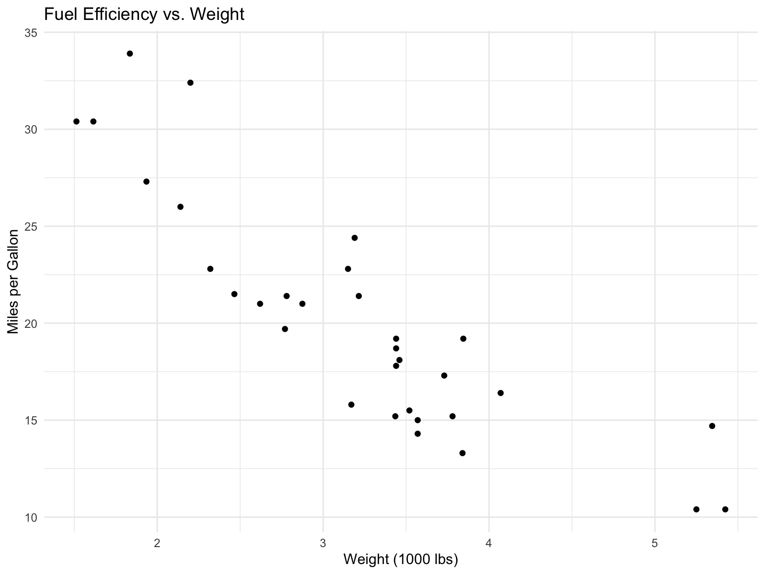
ggplot(mtcars, aes(x = wt, y = mpg)) +geom_point() +labs(title ="Fuel Efficiency vs. Weight",x ="Weight (1000 lbs)",y ="Miles per Gallon" )
Figure 13.5: Relationship between car weight and fuel efficiency
Adding Color and Shape
Map additional variables to aesthetics:
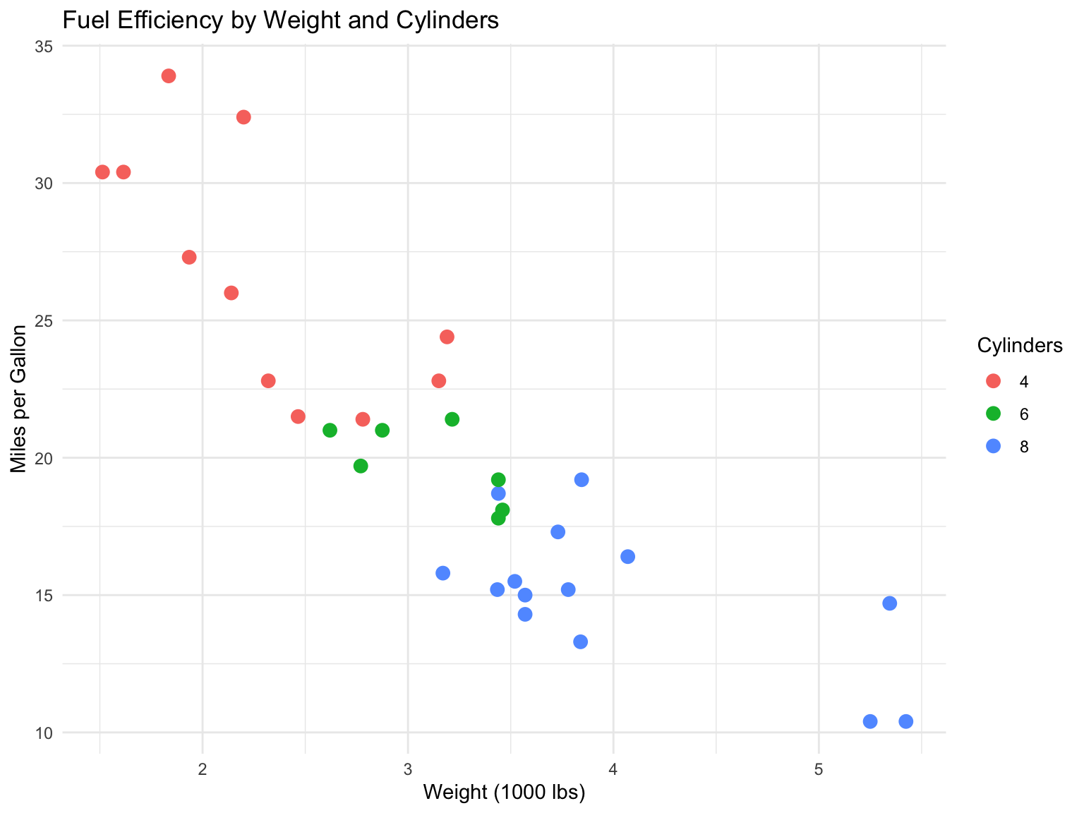
ggplot(mtcars, aes(x = wt, y = mpg, color =factor(cyl))) +geom_point(size =3) +labs(title ="Fuel Efficiency by Weight and Cylinders",x ="Weight (1000 lbs)",y ="Miles per Gallon",color ="Cylinders" )
Figure 13.6: Scatter plot with color representing cylinders
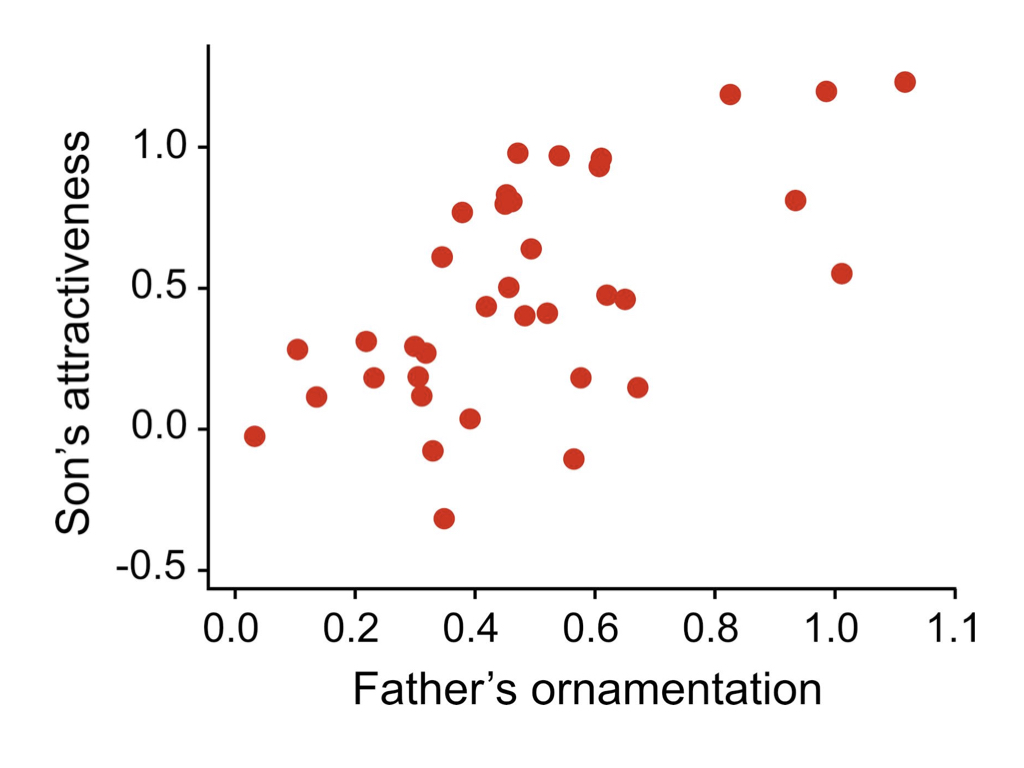
Figure 13.7: Scatter plots are excellent for exploring relationships between two continuous variables. This example shows a positive correlation between two traits, demonstrating how scatter plots can reveal patterns in biological data.
Mapping vs. Setting Aesthetics
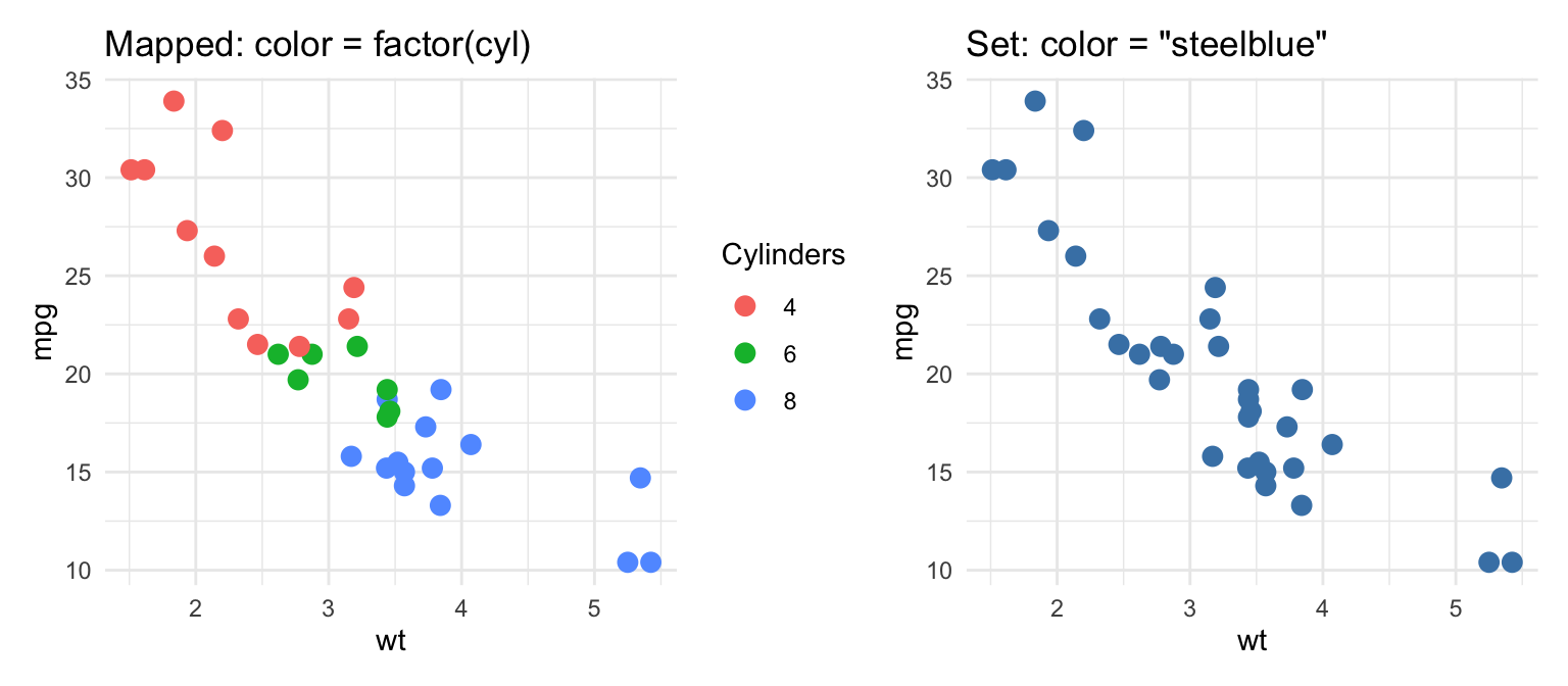
The example above illustrates the single most common ggplot2 confusion. An aesthetic written insideaes() is mapped to a variable: ggplot2 picks a scale, assigns a different value to each level, and draws a legend. An aesthetic written outsideaes(), as a plain argument to the geom, is set to a constant that applies to every observation.
library(patchwork)p_mapped <-ggplot(mtcars, aes(x = wt, y = mpg, color =factor(cyl))) +geom_point(size =3) +labs(title ="Mapped: color = factor(cyl)", color ="Cylinders")p_set <-ggplot(mtcars, aes(x = wt, y = mpg)) +geom_point(size =3, color ="steelblue") +labs(title ="Set: color = \"steelblue\"")p_mapped + p_set
Figure 13.8: Left: colour mapped to a variable inside aes(), producing a legend. Right: colour set to a constant outside aes().
A classic mistake is writing aes(color = "blue"): ggplot2 treats the string "blue" as a one-level variable, maps it to the first colour of the default palette (salmon), and adds a legend labelled “blue”. If you want every point the same colour, keep the argument outside aes(). The same logic applies to size, shape, alpha (transparency, useful for overlapping points), fill, and linetype.
Histograms with geom_histogram()
Histograms show the distribution of a single continuous variable:
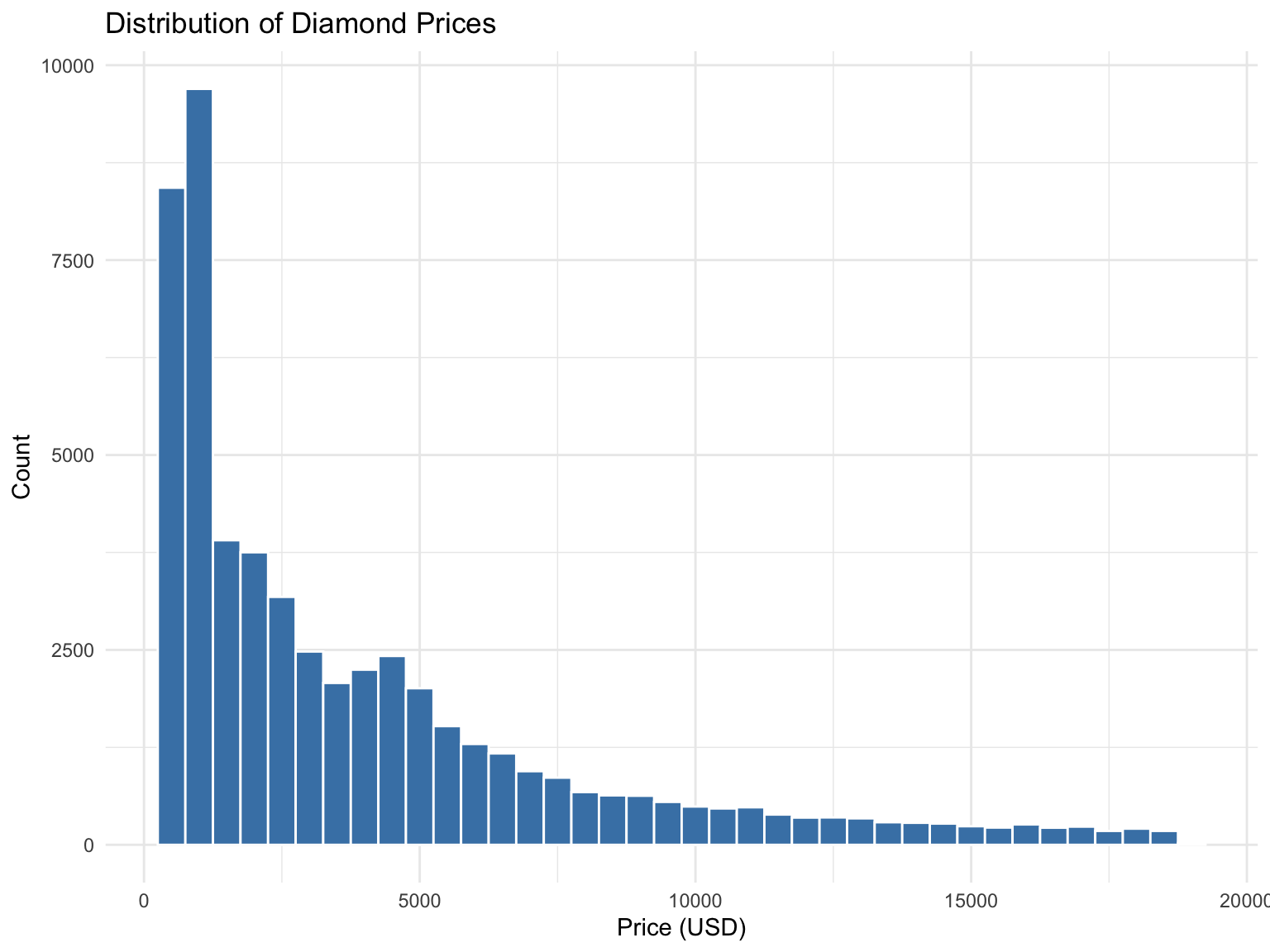
ggplot(diamonds, aes(x = price)) +geom_histogram(binwidth =500, fill ="steelblue", color ="white") +labs(title ="Distribution of Diamond Prices",x ="Price (USD)",y ="Count" )
Figure 13.9: Distribution of diamond prices
Frequency Polygons with geom_freqpoly()
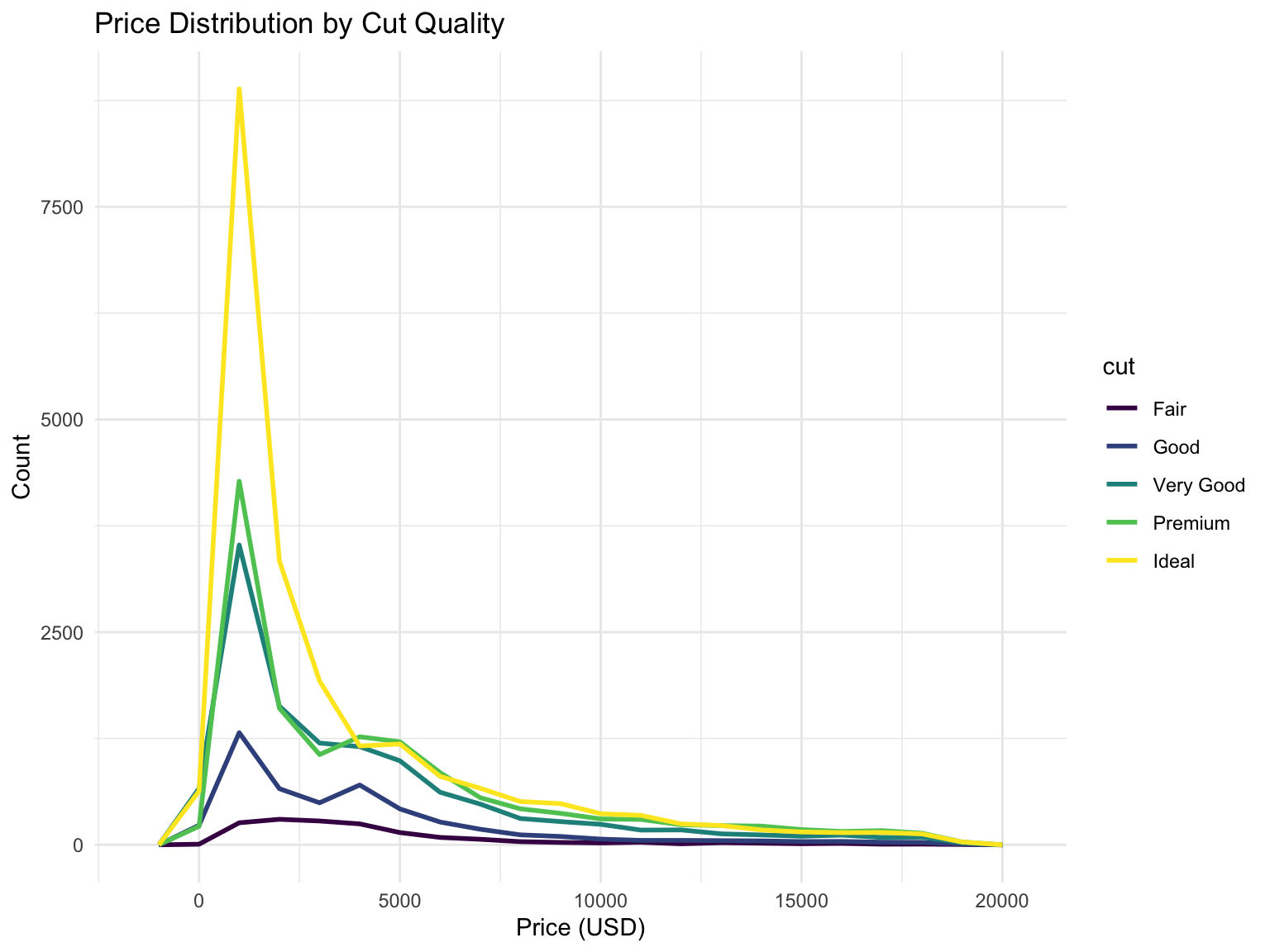
Frequency polygons are an alternative to histograms, showing counts as lines instead of bars. They’re especially useful for comparing multiple distributions:
ggplot(diamonds, aes(x = price, color = cut)) +geom_freqpoly(binwidth =1000, linewidth =1) +labs(title ="Price Distribution by Cut Quality",x ="Price (USD)",y ="Count" )
Figure 13.10: Comparing distributions with frequency polygons
Density Plots with geom_density()
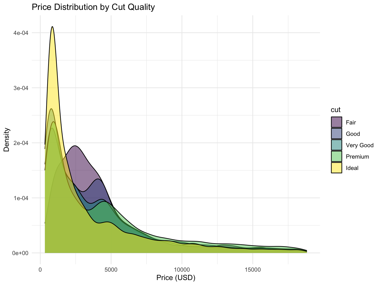
Smoothed version of histograms:
ggplot(diamonds, aes(x = price, fill = cut)) +geom_density(alpha =0.5) +labs(title ="Price Distribution by Cut Quality",x ="Price (USD)",y ="Density" )
Figure 13.11: Density plot comparing distributions by cut quality
Box Plots with geom_boxplot()
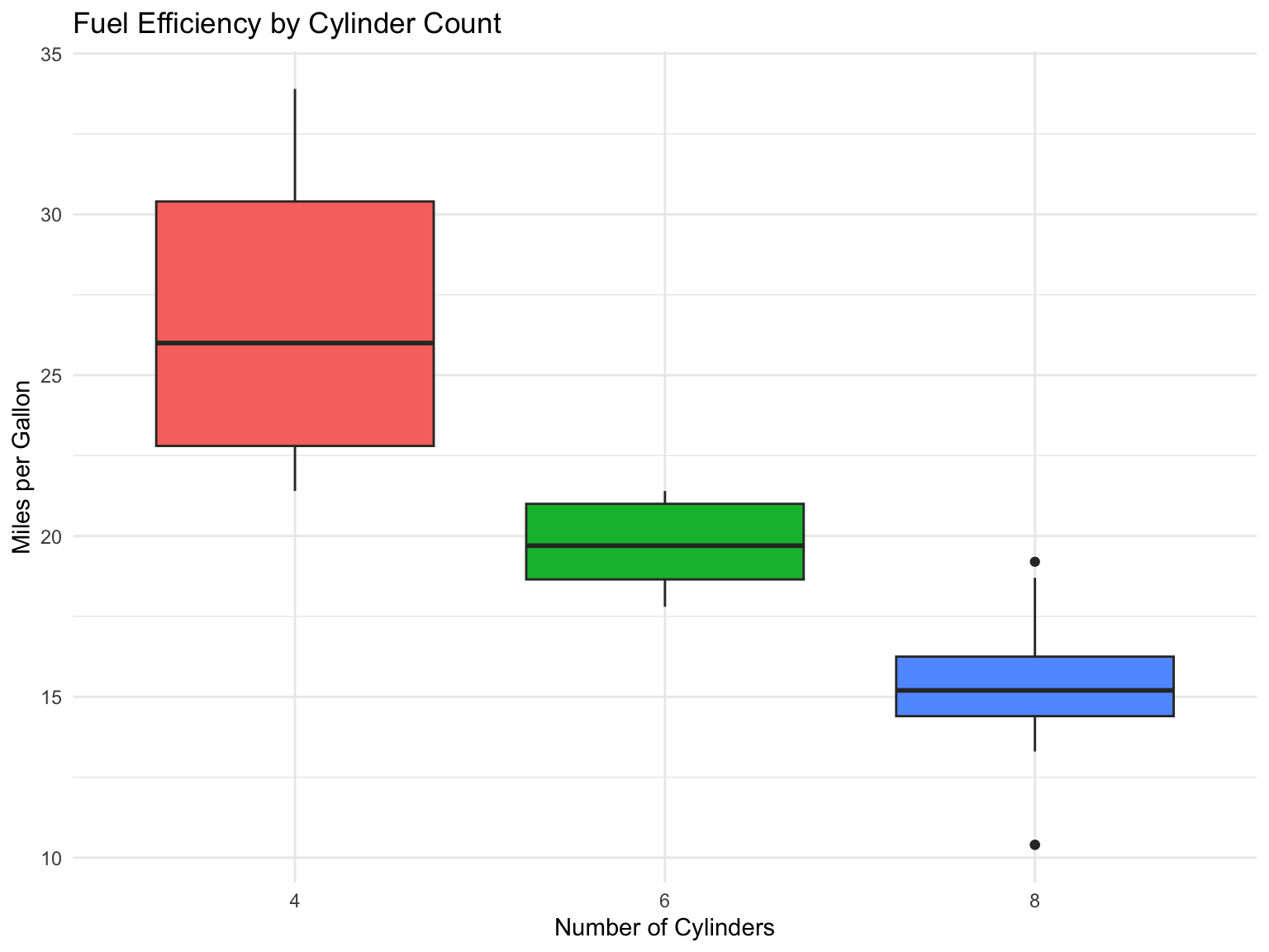
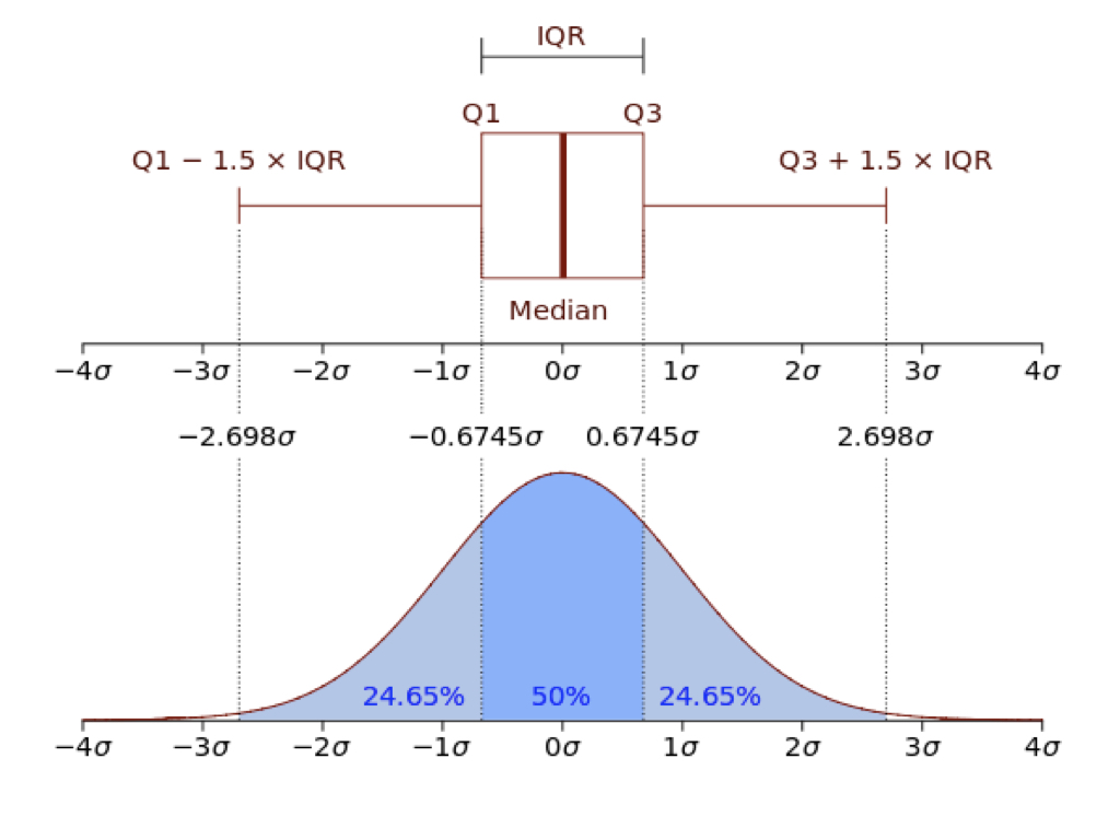
Box plots show distribution summaries (Figure 13.13) and are excellent for comparisons:
ggplot(mtcars, aes(x =factor(cyl), y = mpg, fill =factor(cyl))) +geom_boxplot(show.legend =FALSE) +labs(title ="Fuel Efficiency by Cylinder Count",x ="Number of Cylinders",y ="Miles per Gallon" )
Figure 13.12: Fuel efficiency by number of cylinders
Figure 13.13: Anatomy of a box plot
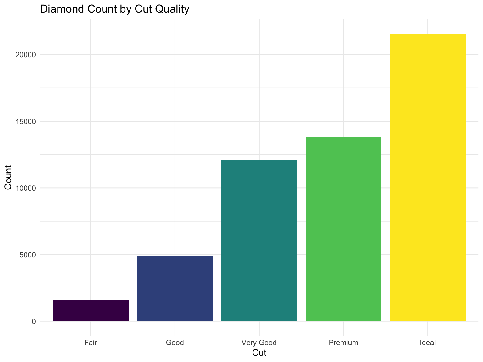
Bar Charts with geom_bar() and geom_col()
Use geom_bar() for counts and geom_col() for values:
ggplot(diamonds, aes(x = cut, fill = cut)) +geom_bar(show.legend =FALSE) +labs(title ="Diamond Count by Cut Quality",x ="Cut",y ="Count" )
Figure 13.14: Count of diamonds by cut quality
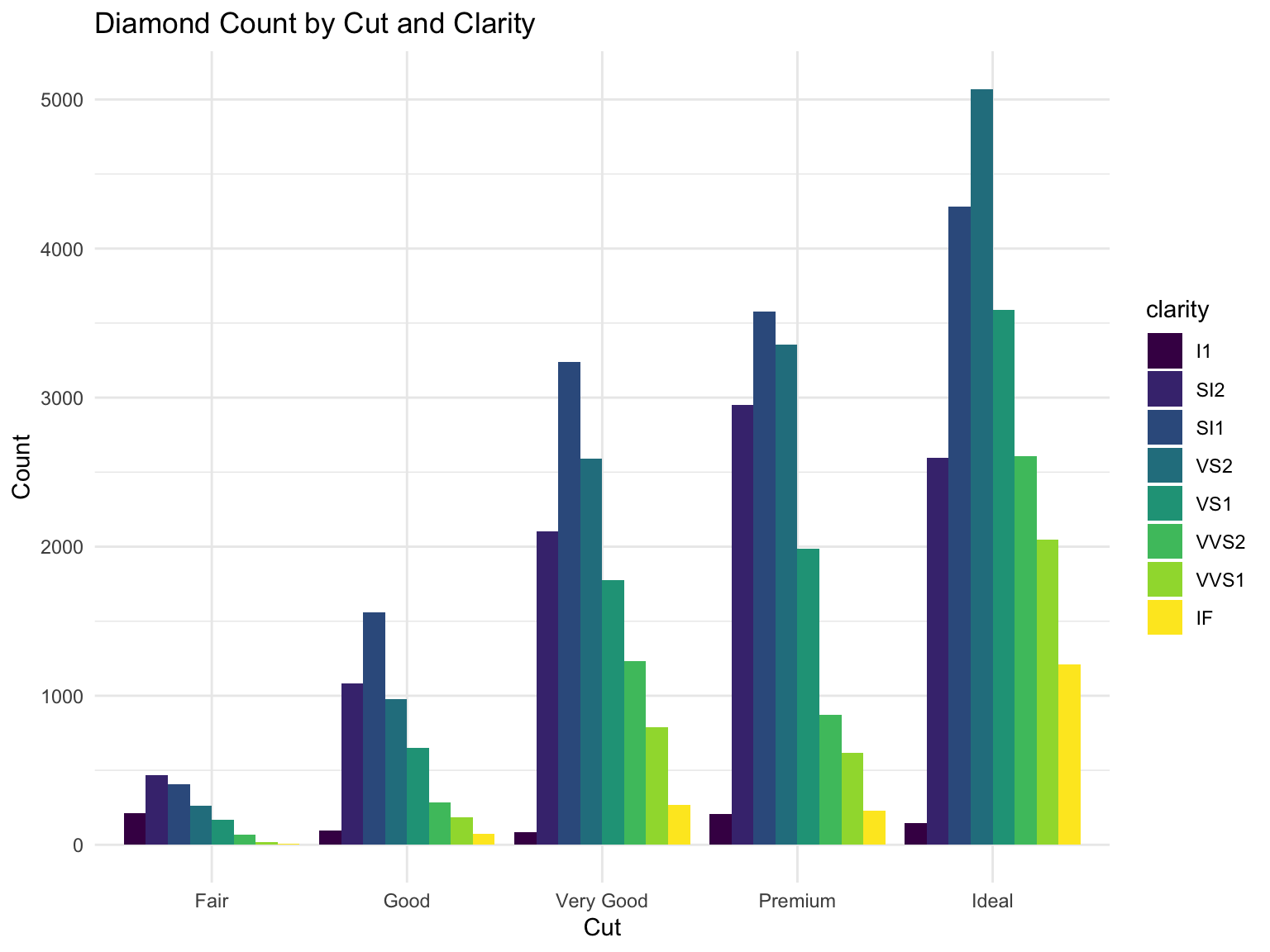
Grouped Bar Charts with position = "dodge"
When you have two categorical variables, use position = "dodge" to place bars side-by-side:
ggplot(diamonds, aes(x = cut, fill = clarity)) +geom_bar(position ="dodge") +labs(title ="Diamond Count by Cut and Clarity",x ="Cut",y ="Count" )
Figure 13.15: Grouped bar chart showing cut quality by clarity
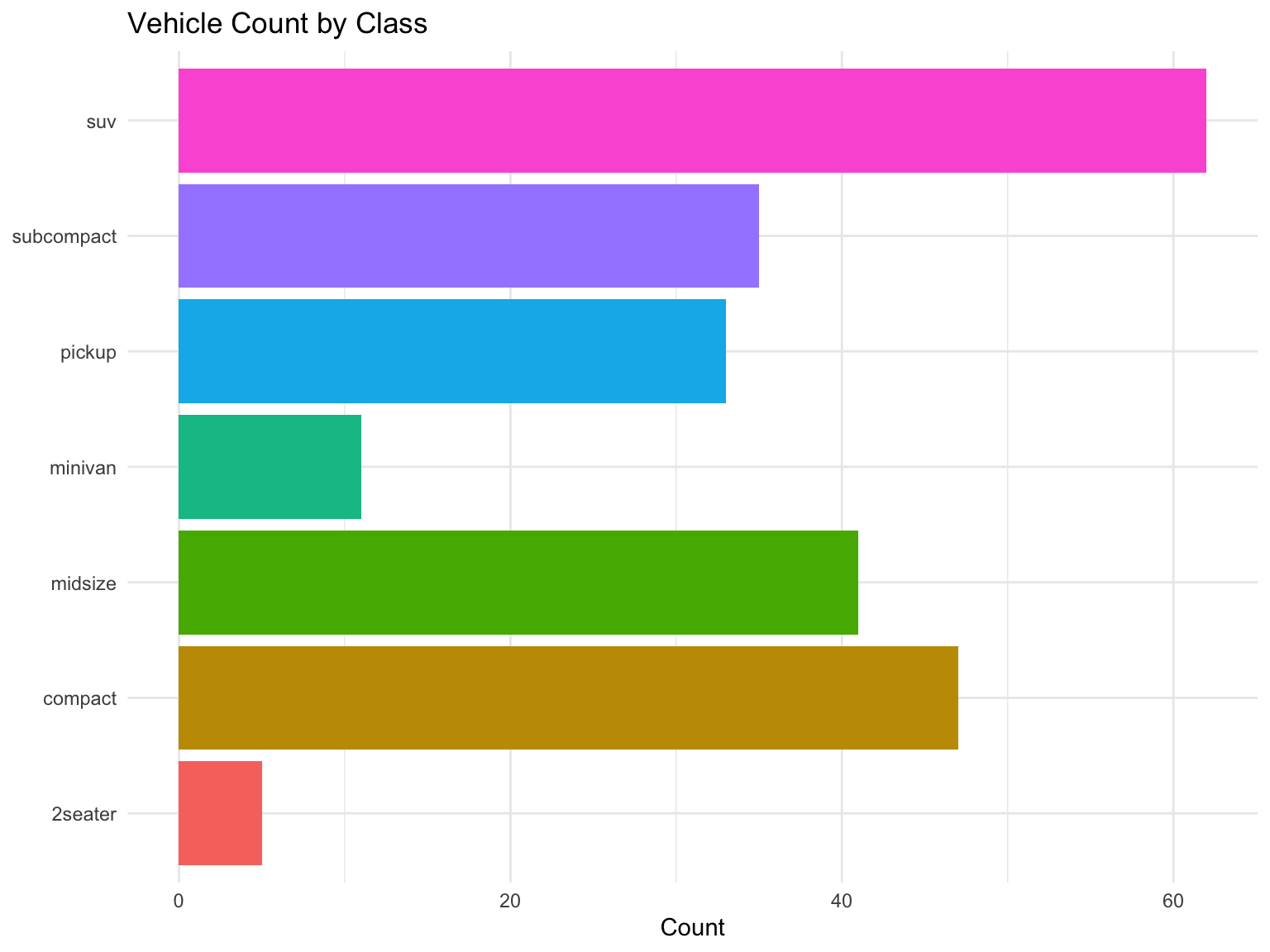
Horizontal Bar Charts with coord_flip()
For long category names or many categories, flip the coordinates to make labels readable:
ggplot(mpg, aes(x = class, fill = class)) +geom_bar(show.legend =FALSE) +coord_flip() +labs(title ="Vehicle Count by Class",x =NULL,y ="Count" )
Figure 13.16: Horizontal bar chart for better label readability
Line Plots with geom_line()
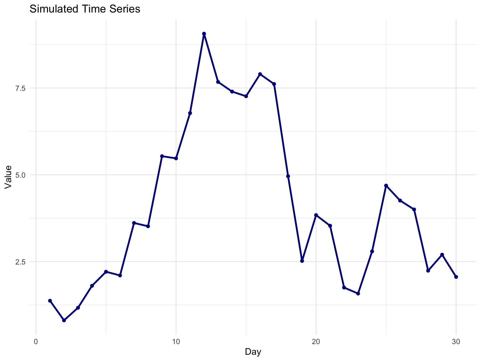
Line plots are ideal for time series or connected observations:
# Create sample time series dataset.seed(42)time_data <-tibble(day =1:30,value =cumsum(rnorm(30)))ggplot(time_data, aes(x = day, y = value)) +geom_line(color ="darkblue", linewidth =1) +geom_point(color ="darkblue") +labs(title ="Simulated Time Series",x ="Day",y ="Value" )
Figure 13.17: Example line plot
13.6 Combining Geoms
Layer multiple geoms to create richer visualizations:
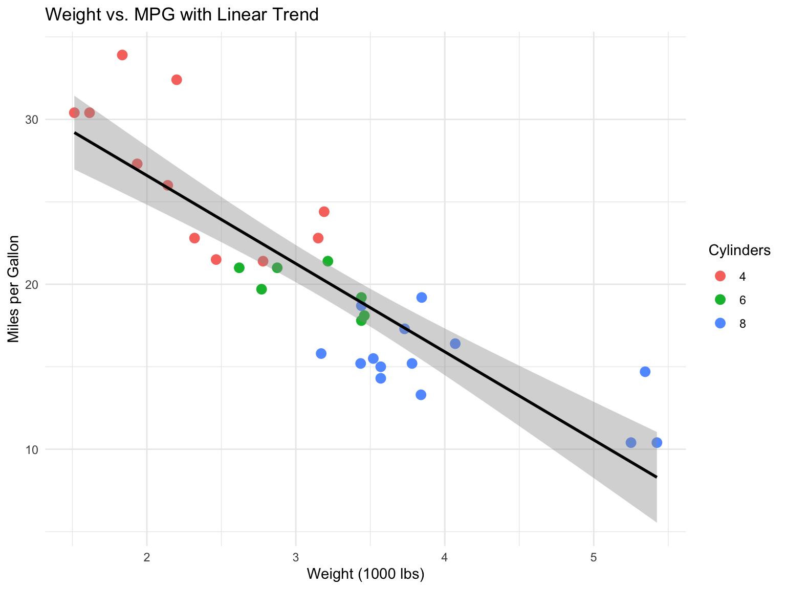
ggplot(mtcars, aes(x = wt, y = mpg)) +geom_point(aes(color =factor(cyl)), size =3) +geom_smooth(method ="lm", se =TRUE, color ="black") +labs(title ="Weight vs. MPG with Linear Trend",x ="Weight (1000 lbs)",y ="Miles per Gallon",color ="Cylinders" )
Figure 13.18: Scatter plot with trend line
Notice that the colour mapping is placed inside geom_point() rather than in ggplot(), so it applies only to the points; the trend line is drawn once for all the data. Aesthetics in ggplot() are inherited by every layer, while aesthetics in a geom apply to that layer alone. With no method argument, geom_smooth() fits a LOESS curve (or a GAM for large data) and shades its confidence band; method = "lm" asks for a straight line instead.
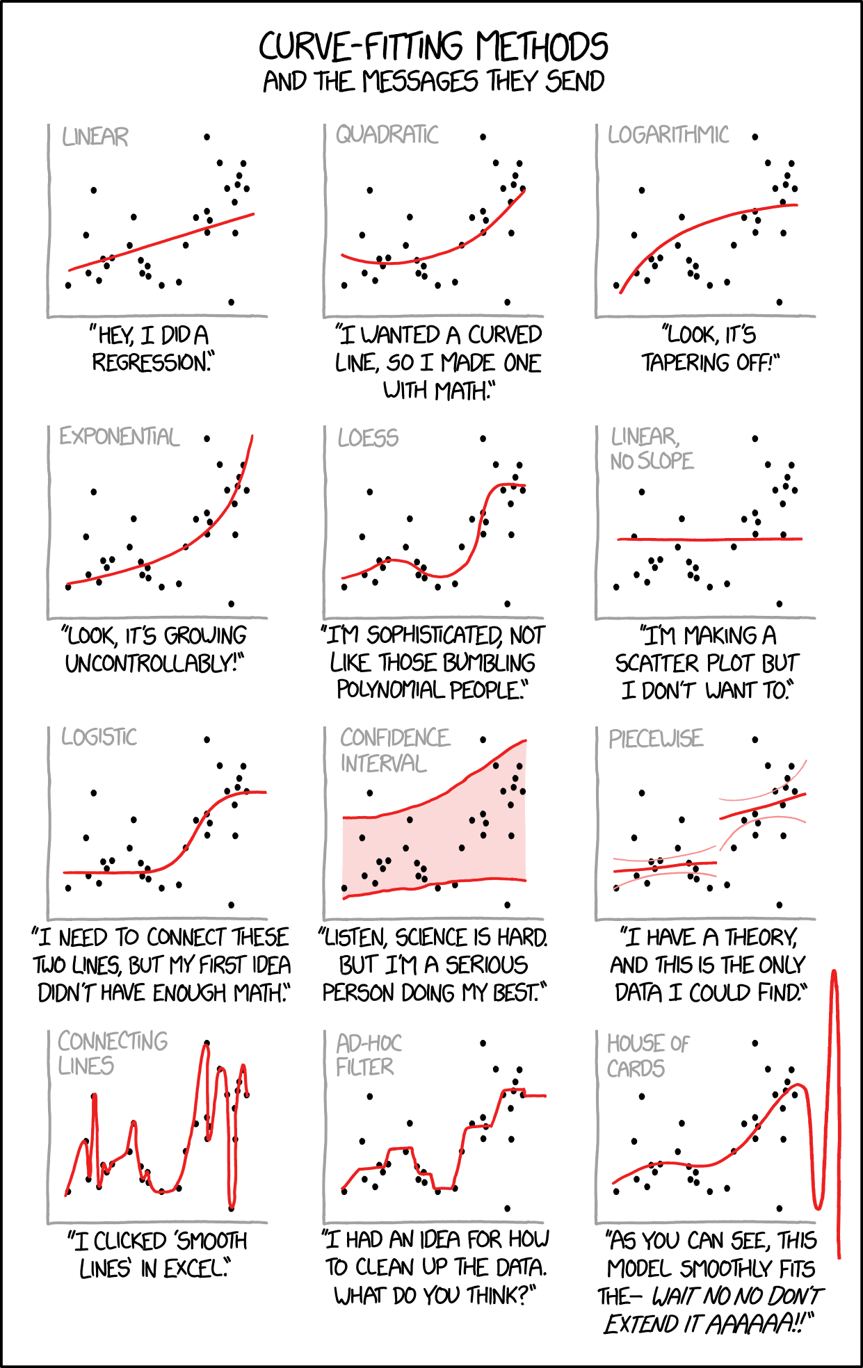
WarningChoose Appropriate Models
When adding trend lines or smoothing to your data, choose methods that match your data structure and research questions. Overfitting with overly complex models can obscure real patterns rather than reveal them (Figure 13.19).
Figure 13.19: Different curve-fitting methods send different messages about your data. Choose methods that match your hypotheses and data characteristics, not just what makes the prettiest curve. Source: xkcd.com
13.7 Faceting: Small Multiples
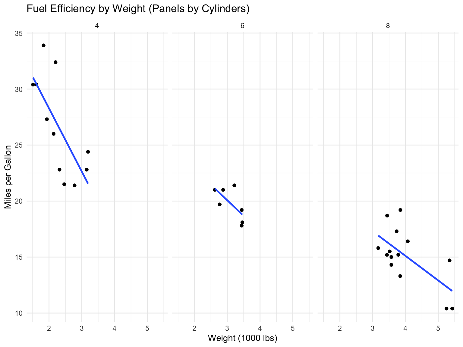
Faceting creates separate panels for subsets of data. The result is a set of small multiples—the same chart repeated for each subset—which Edward Tufte called “the best design solution for a wide range of problems in data presentation.” Small multiples work because the eye can scan and compare panels quickly, every panel shares the same axes so comparisons are fair, and patterns or outliers stand out through repetition. Faceting is usually the best way to add a third (categorical) variable to a plot, and it scales far better than piling more colours and shapes into one panel.
facet_wrap() for One Variable
ggplot(mtcars, aes(x = wt, y = mpg)) +geom_point() +geom_smooth(method ="lm", se =FALSE) +facet_wrap(~cyl) +labs(title ="Fuel Efficiency by Weight (Panels by Cylinders)",x ="Weight (1000 lbs)",y ="Miles per Gallon" )
Figure 13.20: MPG vs weight, faceted by cylinder count
facet_grid() for Two Variables
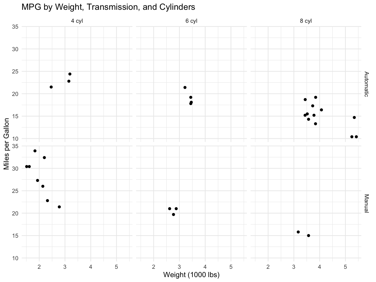
ggplot(mtcars, aes(x = wt, y = mpg)) +geom_point() +facet_grid(am ~ cyl, labeller =labeller(am =c("0"="Automatic", "1"="Manual"),cyl =c("4"="4 cyl", "6"="6 cyl", "8"="8 cyl") )) +labs(title ="MPG by Weight, Transmission, and Cylinders",x ="Weight (1000 lbs)",y ="Miles per Gallon" )
Figure 13.21: Two-dimensional faceting
By default every panel shares the same axis limits, which is what makes comparison fair. When the subsets have very different ranges, scales = "free" (or "free_x", "free_y") lets each panel choose its own; use it deliberately, because it removes exactly the shared reference that small multiples rely on.
13.8 Customizing Your Plots
Labels and Titles
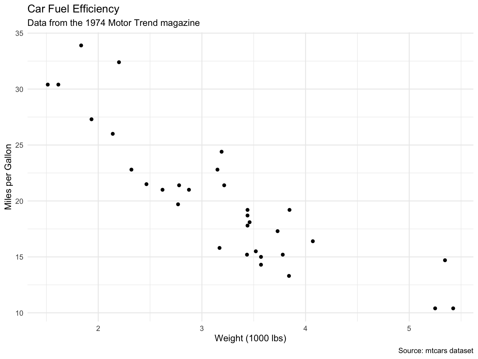
ggplot(mtcars, aes(x = wt, y = mpg)) +geom_point() +labs(title ="Car Fuel Efficiency",subtitle ="Data from the 1974 Motor Trend magazine",x ="Weight (1000 lbs)",y ="Miles per Gallon",caption ="Source: mtcars dataset" )
Figure 13.22: Plot with comprehensive labels
Themes
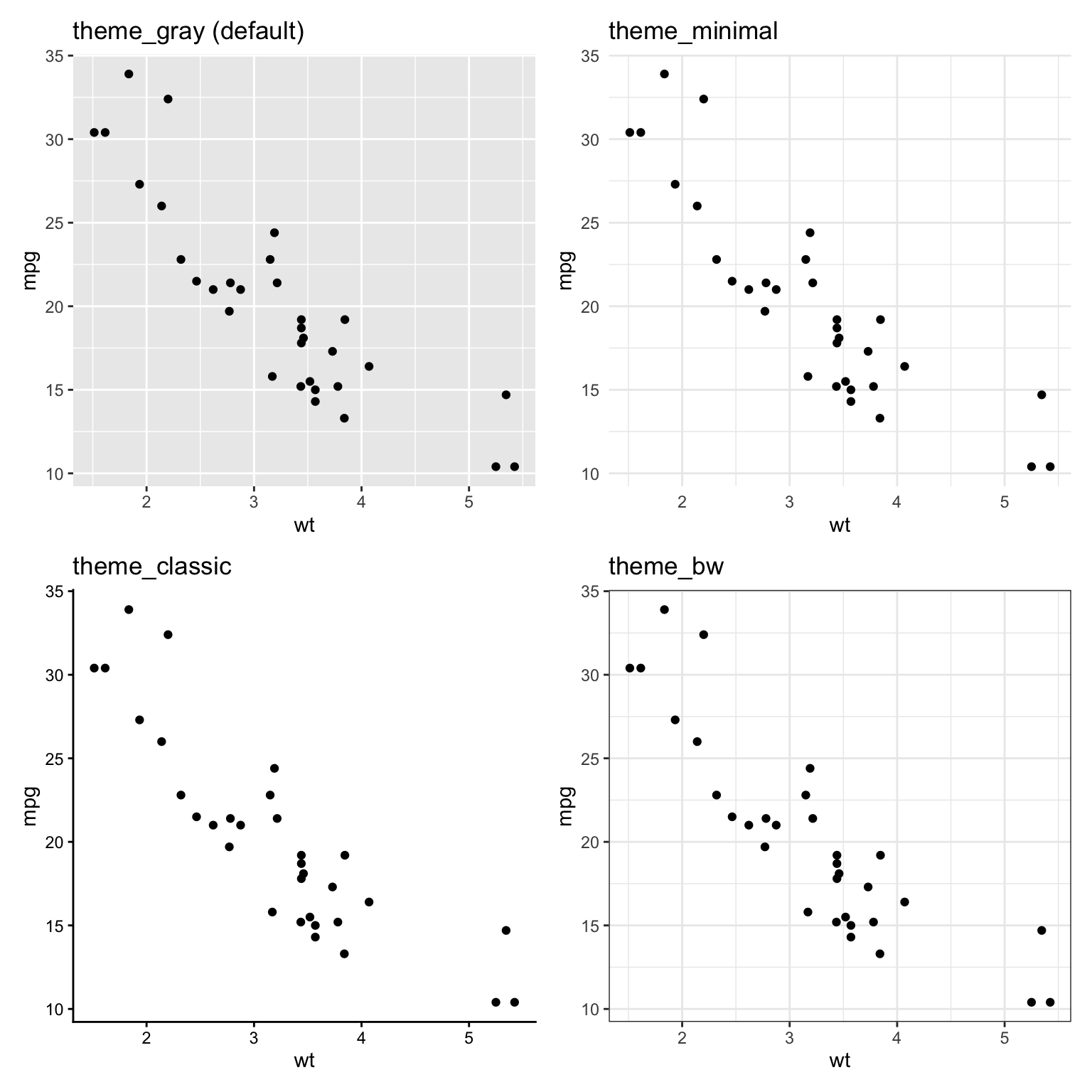
ggplot2 includes several built-in themes:
library(patchwork)p <-ggplot(mtcars, aes(x = wt, y = mpg)) +geom_point() +labs(title ="")p1 <- p +theme_gray() +labs(title ="theme_gray (default)")p2 <- p +theme_minimal() +labs(title ="theme_minimal")p3 <- p +theme_classic() +labs(title ="theme_classic")p4 <- p +theme_bw() +labs(title ="theme_bw")(p1 + p2) / (p3 + p4)
Figure 13.23: Comparison of ggplot2 themes
Other built-in themes include theme_light(), theme_dark(), and theme_void() (no axes at all, for maps and diagrams); the ggthemes package adds many more, including Tufte- and Economist-style themes. theme_set() at the top of a script or document, as in this chapter’s setup chunk, applies one theme to every plot that follows.
Fine-Tuning with theme()
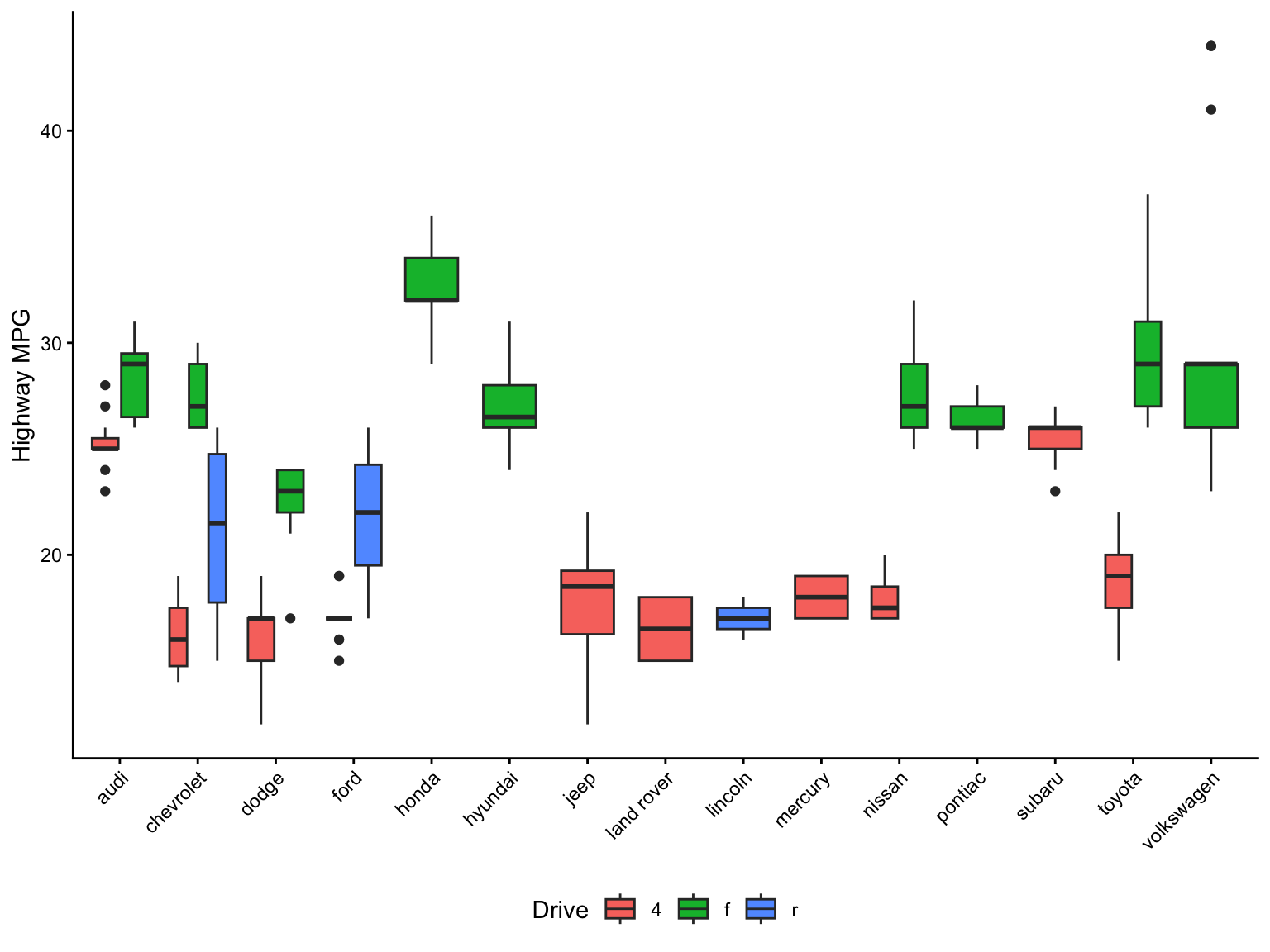
Complete themes set everything at once; theme() adjusts individual elements. The most frequent use is rotating axis labels when categories have long names, followed by moving or removing the legend:
ggplot(mpg, aes(x = manufacturer, y = hwy, fill = drv)) +geom_boxplot() +labs(x =NULL, y ="Highway MPG", fill ="Drive") +theme_classic() +theme(axis.text.x =element_text(angle =45, hjust =1),legend.position ="bottom" )
Figure 13.24: Rotated axis labels and a bottom legend via theme()
Elements are named by what they control (axis.text.x, panel.grid.minor, plot.title, strip.text) and are set with element_text(), element_line(), element_rect(), or element_blank() to remove them. theme() must come after a complete theme such as theme_classic(), otherwise the complete theme overwrites your tweaks.
Log Scales
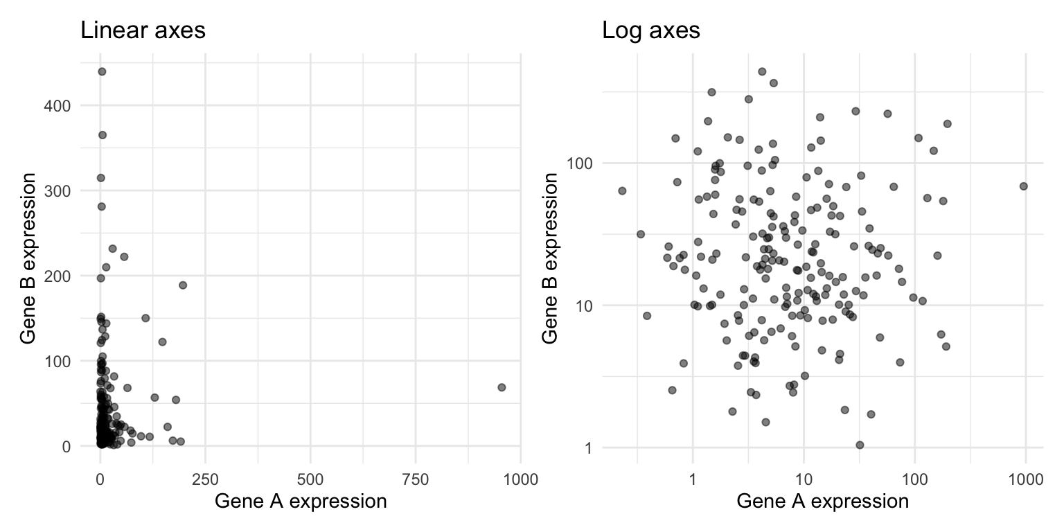
Many biological quantities—gene expression, cell counts, concentrations, population sizes—span several orders of magnitude and are strongly right-skewed. On a linear axis a handful of large values squash everything else into a corner. scale_x_log10() and scale_y_log10() transform the axis while keeping the tick labels in the original units:
set.seed(123)expression_sim <-tibble(gene_a =rlnorm(200, meanlog =2, sdlog =1.5),gene_b =rlnorm(200, meanlog =3, sdlog =1.2))p_raw <-ggplot(expression_sim, aes(x = gene_a, y = gene_b)) +geom_point(alpha =0.5) +labs(title ="Linear axes", x ="Gene A expression", y ="Gene B expression")p_log <- p_raw +scale_x_log10() +scale_y_log10() +labs(title ="Log axes")p_raw + p_log
Figure 13.25: The same simulated expression data on linear axes (left) and log axes (right)
Reach for a log scale when the data span several orders of magnitude, when relationships are multiplicative (fold changes, ratios), or when a distribution has a long right tail. Label the axis so readers know the scale is transformed, and remember that zero and negative values cannot be shown on a log axis (log1p() or a pseudo-log scale, scale_y_continuous(transform = "pseudo_log"), handles counts that include zero).
Color Scales
Colour is the most powerful and the most misused aesthetic. The right scale depends on what kind of variable is mapped to it:
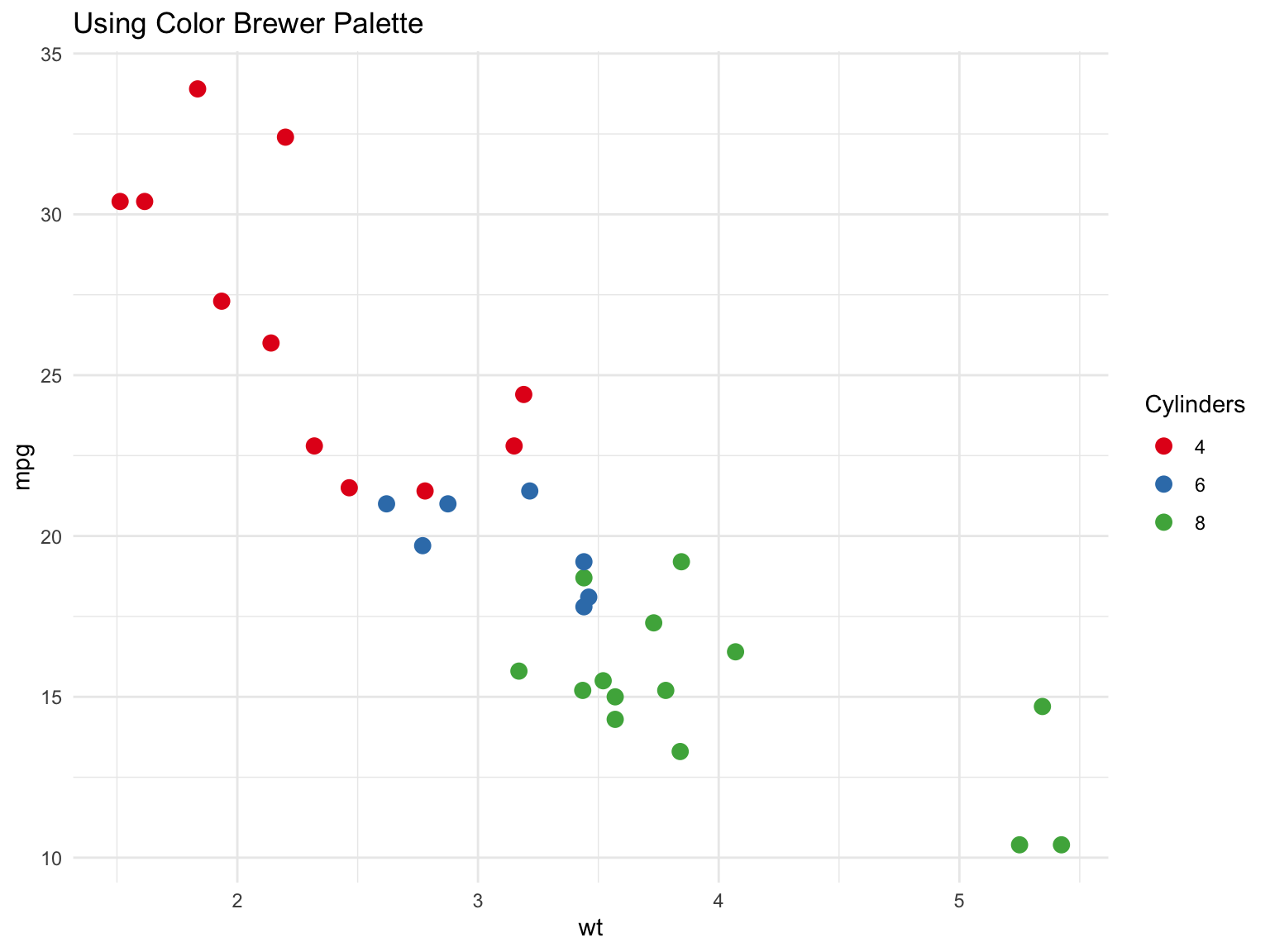
Qualitative scales, for categories with no order: distinct hues of similar brightness (scale_color_brewer(palette = "Set1"), scale_color_viridis_d())
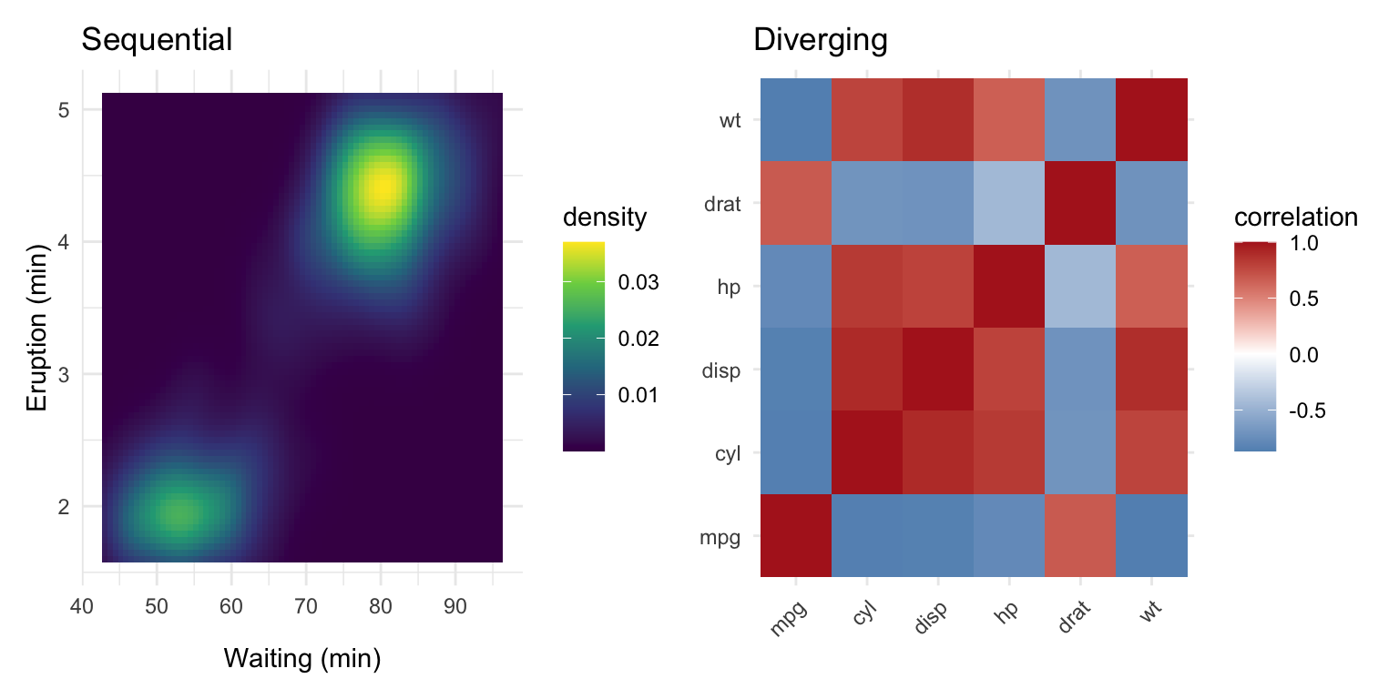
Sequential scales, for ordered or continuous values running from low to high: one hue varying in lightness (scale_fill_viridis_c(), scale_fill_gradient())
Diverging scales, for values with a meaningful midpoint such as zero or a log fold change of 0: two hues diverging from a neutral centre (scale_fill_gradient2())
ggplot(mtcars, aes(x = wt, y = mpg, color =factor(cyl))) +geom_point(size =3) +scale_color_brewer(palette ="Set1") +labs(title ="Using Color Brewer Palette",color ="Cylinders" ) +theme_minimal()
Figure 13.26: A qualitative ColorBrewer palette for an unordered categorical variable
p_seq <-ggplot(faithfuld, aes(waiting, eruptions, fill = density)) +geom_tile() +scale_fill_viridis_c() +labs(title ="Sequential", x ="Waiting (min)", y ="Eruption (min)")corr_df <-cor(mtcars[, 1:6]) |>as.table() |>as.data.frame() |>setNames(c("var1", "var2", "correlation"))p_div <-ggplot(corr_df, aes(var1, var2, fill = correlation)) +geom_tile() +scale_fill_gradient2(low ="steelblue", mid ="white", high ="firebrick",midpoint =0) +labs(title ="Diverging", x =NULL, y =NULL) +theme(axis.text.x =element_text(angle =45, hjust =1))p_seq + p_div
Figure 13.27: A sequential viridis scale for density (left) and a diverging scale centred on zero for correlations (right)
The scale_* function names follow a pattern: the aesthetic (color/colour or fill), then the palette family, then _d for discrete or _c for continuous data. Using a continuous scale on a factor, or vice versa, is a frequent source of errors.
WarningAvoid Rainbow Scales
Rainbow colour maps (MATLAB’s old “jet”, or rainbow() in base R) are not perceptually uniform: yellow looks brighter than blue, so equal steps in the data do not look like equal steps in colour, and sharp hue changes create boundaries that are not in the data. They are also unreadable for colour-blind viewers. Use viridis, plasma, or another perceptually uniform scale for continuous data.
13.9 Data Visualization Best Practices
Good data visualization communicates clearly and honestly. Edward Tufte, whose The Visual Display of Quantitative Information(Tufte, 1983) remains the standard reference, put it this way:
“Graphical excellence is that which gives to the viewer the greatest number of ideas in the shortest time with the least ink in the smallest space.”
His principles of graphical excellence are the ones that follow: show the data; encourage the eye to compare differences; represent magnitudes honestly; draw graphical elements clearly, minimizing clutter; and make displays easy to interpret.
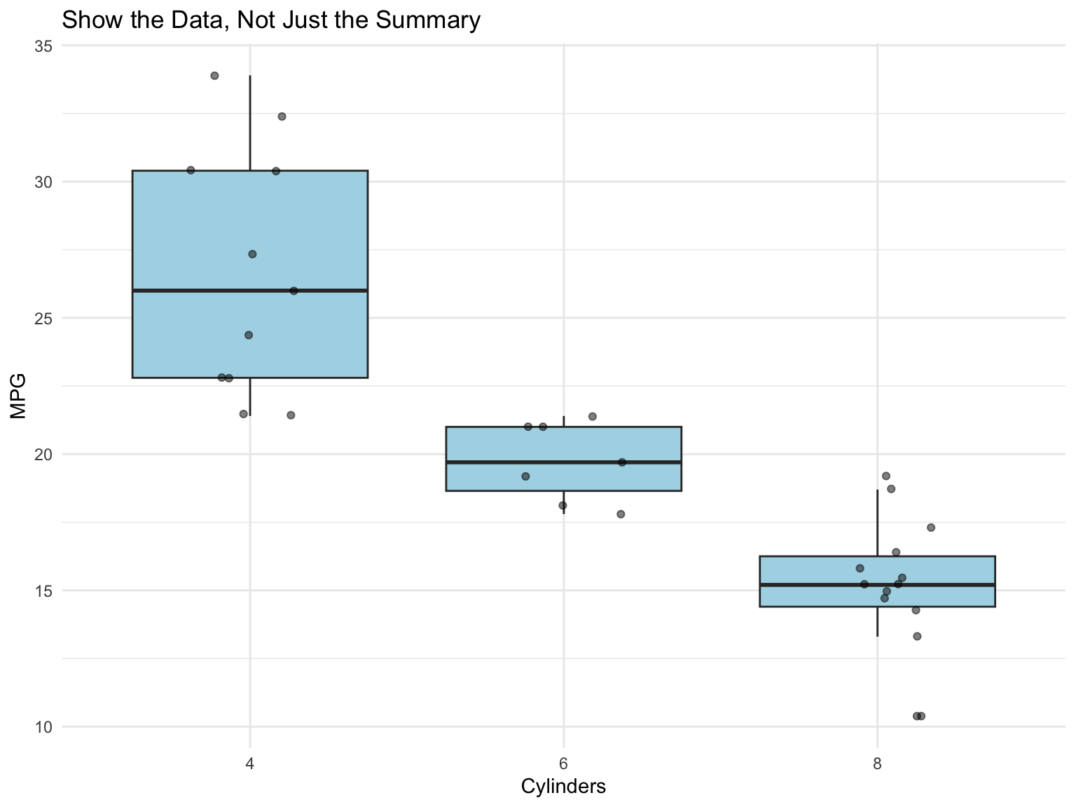
Show the Data
“Above all else show the data.” Don’t hide your data behind summaries when individual points are informative:
ggplot(mtcars, aes(x =factor(cyl), y = mpg)) +geom_boxplot(outlier.shape =NA, fill ="lightblue") +geom_jitter(width =0.2, alpha =0.5) +labs(title ="Show the Data, Not Just the Summary",x ="Cylinders",y ="MPG" )
Figure 13.28: Showing raw data with summary statistics
Use Position and Length for Precision
Every chart encodes numbers as visual cues—position, length, angle, area, colour—and we do not read all cues equally well. Cleveland and McGill’s experiments (Cleveland & McGill, 1984) ranked them from most to least accurately perceived:
Position along a common scale (scatter plots, dot plots)
Position along non-aligned scales (small multiples)
Length (bar charts)
Angle and slope (pie charts, some line charts)
Area (bubble charts, treemaps)
Volume (3D charts—avoid)
Colour saturation and hue (heat maps, choropleth maps)
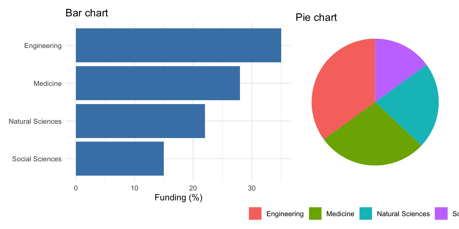
Encode the quantity you most want the reader to compare using position or length, and keep colour and area for secondary information. This is why a bar chart beats a pie chart for the same data (Figure 13.29): the bars ask the eye to compare lengths against a common baseline, the pie asks it to compare angles.
funding <-tibble(field =c("Engineering", "Medicine", "Natural Sciences", "Social Sciences"),pct =c(35, 28, 22, 15))p_bar <-ggplot(funding, aes(x =reorder(field, pct), y = pct)) +geom_col(fill ="steelblue") +coord_flip() +labs(title ="Bar chart", x =NULL, y ="Funding (%)")p_pie <-ggplot(funding, aes(x ="", y = pct, fill = field)) +geom_col(width =1) +coord_polar("y") +labs(title ="Pie chart", fill =NULL) +theme_void() +theme(legend.position ="bottom")p_bar + p_pie
Figure 13.29: The same four values as a bar chart (lengths on a common scale) and a pie chart (angles): the ranking is instant on the left and requires effort on the right
WarningAvoid Pie Charts
Pie charts make comparisons difficult because humans are poor at judging angles, and they become unreadable beyond a handful of categories. Use bar charts (or dot plots) instead for categorical comparisons. Note that a pie chart in ggplot2 is literally a stacked bar in polar coordinates (coord_polar()), which shows how the grammar composes.
Order by Meaningful Values
By default, R orders categorical variables alphabetically, which is rarely meaningful. Use reorder() to order by a numeric value instead (the forcats tools in Section 14.7.2 do the same job for factors):
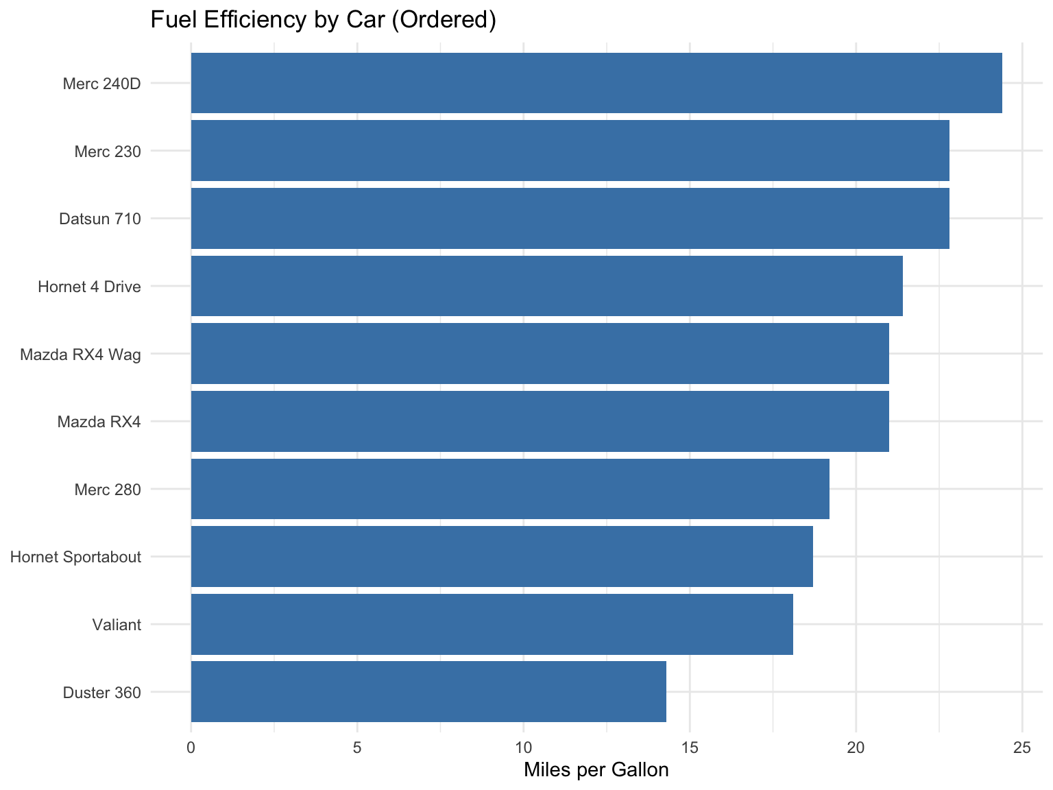
# Calculate mean mpg by manufacturermtcars_summary <- mtcars |>mutate(car =rownames(mtcars)) |>slice_head(n =10) |>mutate(car =reorder(car, mpg)) # Order car names by mpg valuesggplot(mtcars_summary, aes(x = car, y = mpg)) +geom_col(fill ="steelblue") +coord_flip() +labs(title ="Fuel Efficiency by Car (Ordered)",x =NULL,y ="Miles per Gallon" )
Figure 13.30: Ordering categories by value aids comparison
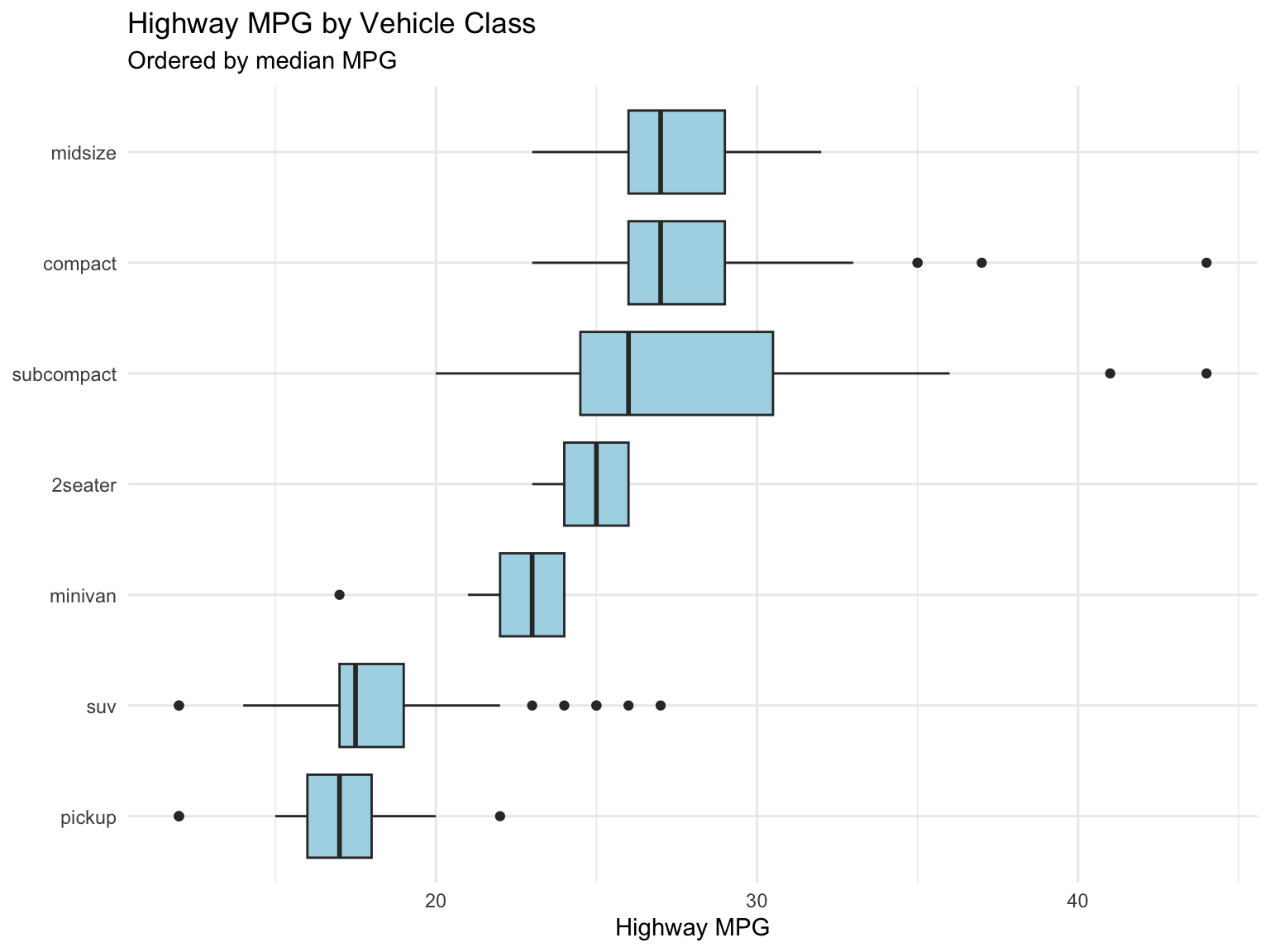
The reorder() function takes a categorical variable and a numeric variable, then reorders the categories by the numeric values. You can also specify a summary function when there are multiple values per category (Figure 13.31):
# Order vehicle class by median highway mpgggplot(mpg, aes(x =reorder(class, hwy, FUN = median), y = hwy)) +geom_boxplot(fill ="lightblue") +coord_flip() +labs(title ="Highway MPG by Vehicle Class",subtitle ="Ordered by median MPG",x =NULL,y ="Highway MPG" )
Figure 13.31: Highway MPG by vehicle class, with classes ordered by their median using reorder()
Represent Magnitudes Honestly: When to Include Zero
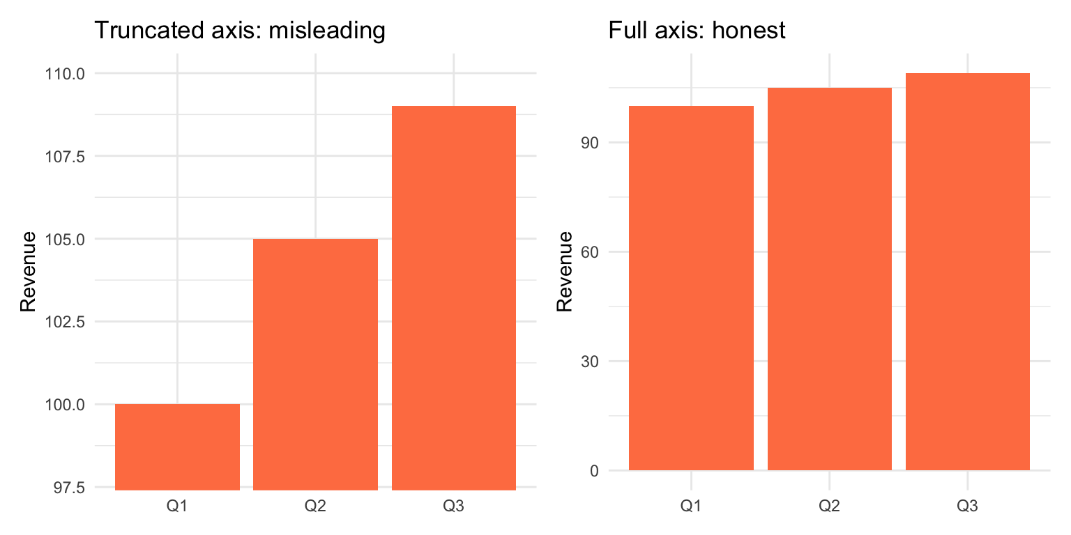
Whether the y-axis must start at zero is a perennial argument, and the answer depends on the encoding. In a bar chart the length of the bar is the magnitude, so a truncated axis misrepresents the data:
sales <-tibble(quarter =c("Q1", "Q2", "Q3"),revenue =c(100, 105, 109))p_trunc <-ggplot(sales, aes(x = quarter, y = revenue)) +geom_col(fill ="coral") +coord_cartesian(ylim =c(98, 110)) +labs(title ="Truncated axis: misleading", x =NULL, y ="Revenue")p_full <-ggplot(sales, aes(x = quarter, y = revenue)) +geom_col(fill ="coral") +labs(title ="Full axis: honest", x =NULL, y ="Revenue")p_trunc + p_full
Figure 13.32: The same three values with a truncated axis (left) and a full axis (right). The left panel makes a 9% difference look like a several-fold one.
Note the mechanics: coord_cartesian(ylim = ...) zooms the view without discarding data, whereas ylim() or scale_y_continuous(limits = ...)drops observations outside the range, and for bars that silently removes every bar taller than the limit. Zoom with coord_cartesian() when you must.
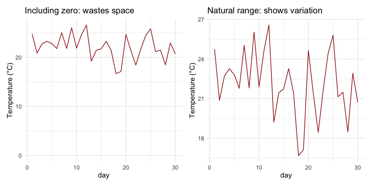
For position-based encodings—line charts and scatter plots—the reader compares positions, not lengths, so forcing zero onto the axis can waste most of the plot and hide the variation you want to show:
set.seed(42)temps <-tibble(day =1:30, temp =rnorm(30, mean =22, sd =2))p_zero <-ggplot(temps, aes(x = day, y = temp)) +geom_line(color ="firebrick") +expand_limits(y =0) +labs(title ="Including zero: wastes space", y ="Temperature (°C)")p_auto <-ggplot(temps, aes(x = day, y = temp)) +geom_line(color ="firebrick") +labs(title ="Natural range: shows variation", y ="Temperature (°C)")p_zero + p_auto
Figure 13.33: Daily temperatures with zero forced onto the axis (left) and on their natural range (right). Zero has no special meaning here, so the right panel is the better plot.
TipThe Zero Rule
Bar charts: always include zero; bar length is the magnitude
Line charts and scatter plots: include zero if it is meaningful for the variable (counts, proportions); otherwise show the natural range of the data
When in doubt: ask whether excluding zero could mislead a reader about the size of a difference. Figure 13.42 shows what happens when it does
Consider Color Blindness
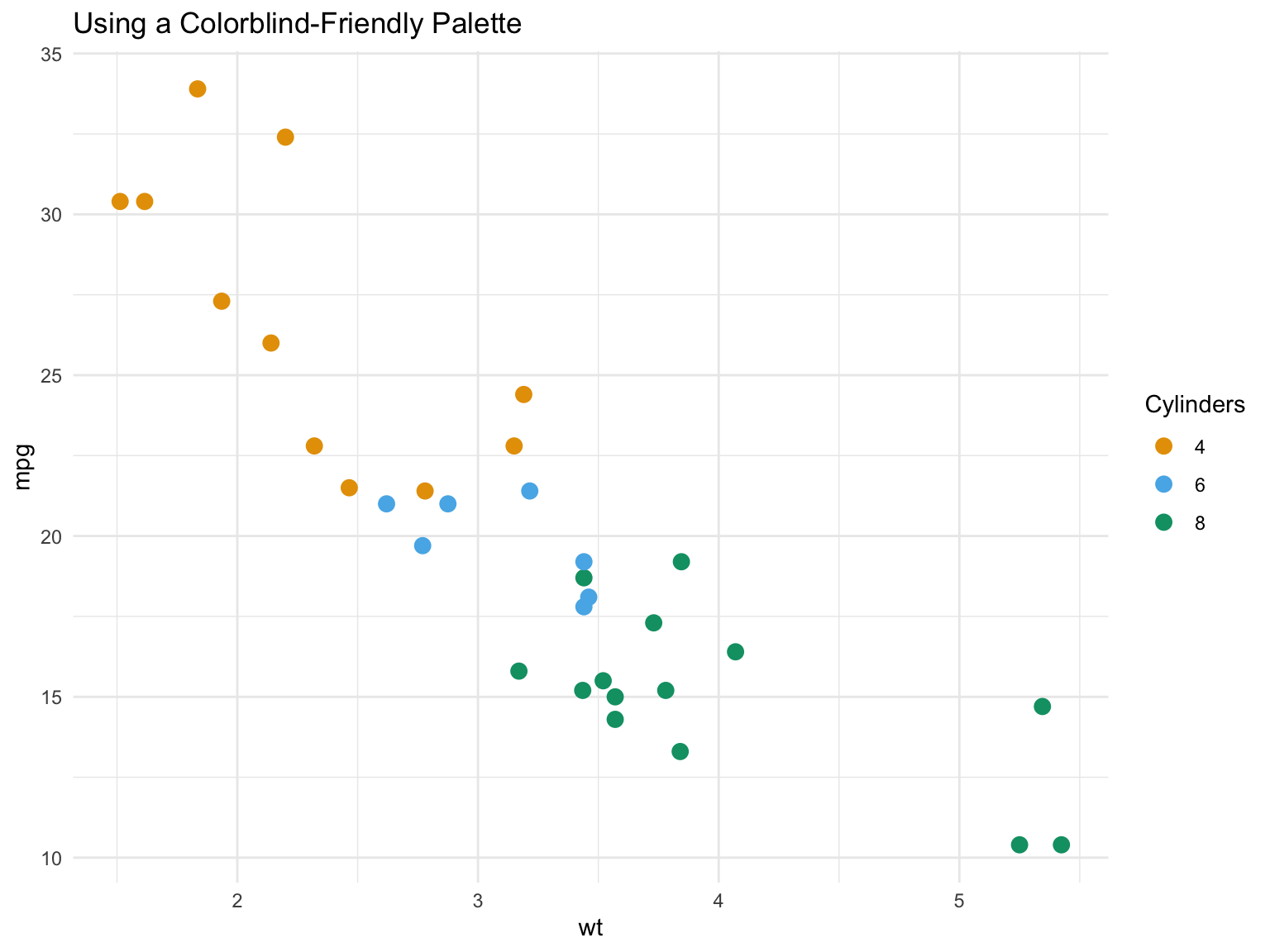
About 8% of men and 0.5% of women have color vision deficiency. Use colorblind-friendly palettes:
# Colorblind-friendly colorscb_palette <-c("#E69F00", "#56B4E9", "#009E73", "#F0E442","#0072B2", "#D55E00", "#CC79A7")ggplot(mtcars, aes(x = wt, y = mpg, color =factor(cyl))) +geom_point(size =3) +scale_color_manual(values = cb_palette) +labs(title ="Using a Colorblind-Friendly Palette",color ="Cylinders" ) +theme_minimal()
Figure 13.34: Colorblind-friendly palette
Tip
The viridis color scales (scale_color_viridis_d(), scale_fill_viridis_c()) are designed to be colorblind-friendly and perceptually uniform, and the palette above (Okabe and Ito’s) is the standard choice for up to eight categories. Avoid red versus green as the only distinguishing feature.
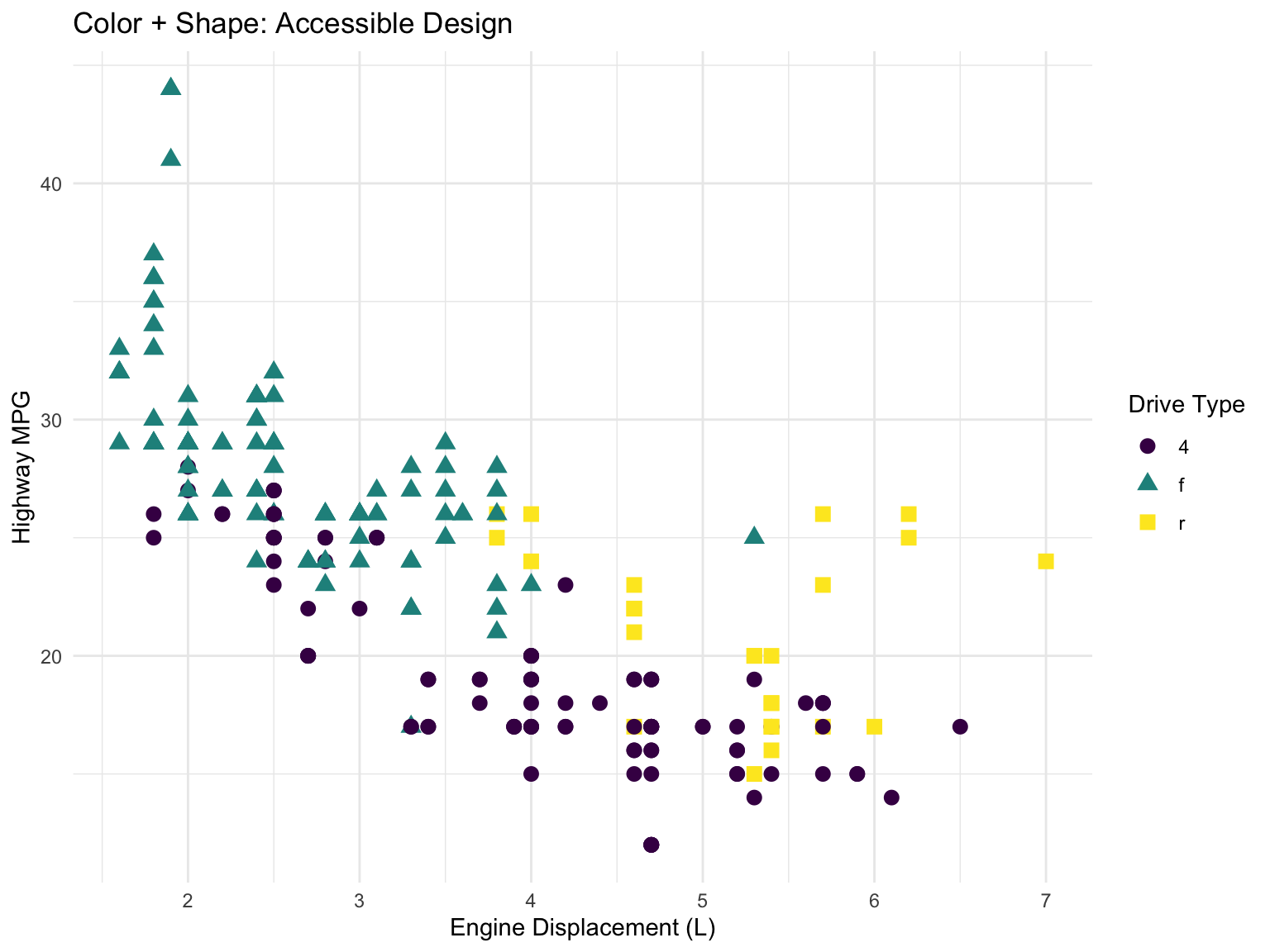
Better still, do not rely on colour alone. Mapping the same variable to both color and shape (or using facets) means the plot still works in greyscale and for every viewer:
Figure 13.35: Redundant encoding: drive type is mapped to both colour and shape, so the groups remain distinguishable without colour
Mapping one variable to two aesthetics produces a single merged legend, as long as both mappings use the same variable and the same legend title.
Avoid Chart Junk
Tufte’s data-ink ratio is the share of a graphic’s ink that actually represents data; the goal is to maximize it. Remove visual elements that convey no information:
Avoid 3D effects, which distort perception without adding anything
Remove unnecessary gridlines, borders, and backgrounds
Don’t use gradient fills for categorical data
Skip decorative elements, clip art, and heavy legends
Two further mistakes are common enough to name. Dual y-axes (two different scales on the left and right of the same panel) are almost always misleading: the relationship between the two scales is arbitrary, and by choosing the ranges you can make any two series appear to track, cross, or diverge. Facet the two variables instead, or plot one against the other. Overplotting—thousands of points drawn on top of one another so the dense regions look like a solid blob—hides the structure you are trying to show; Section 13.10.3 shows the remedies.
13.10 Common Visualization Tasks
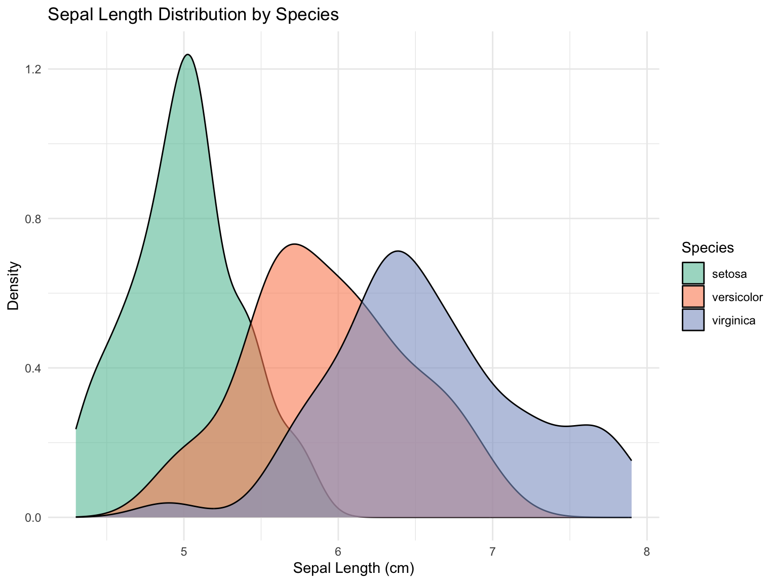
Comparing Distributions
ggplot(iris, aes(x = Sepal.Length, fill = Species)) +geom_density(alpha =0.6) +scale_fill_brewer(palette ="Set2") +labs(title ="Sepal Length Distribution by Species",x ="Sepal Length (cm)",y ="Density" ) +theme_minimal()
Figure 13.36: Comparing distributions with density plots
Before-After Comparisons
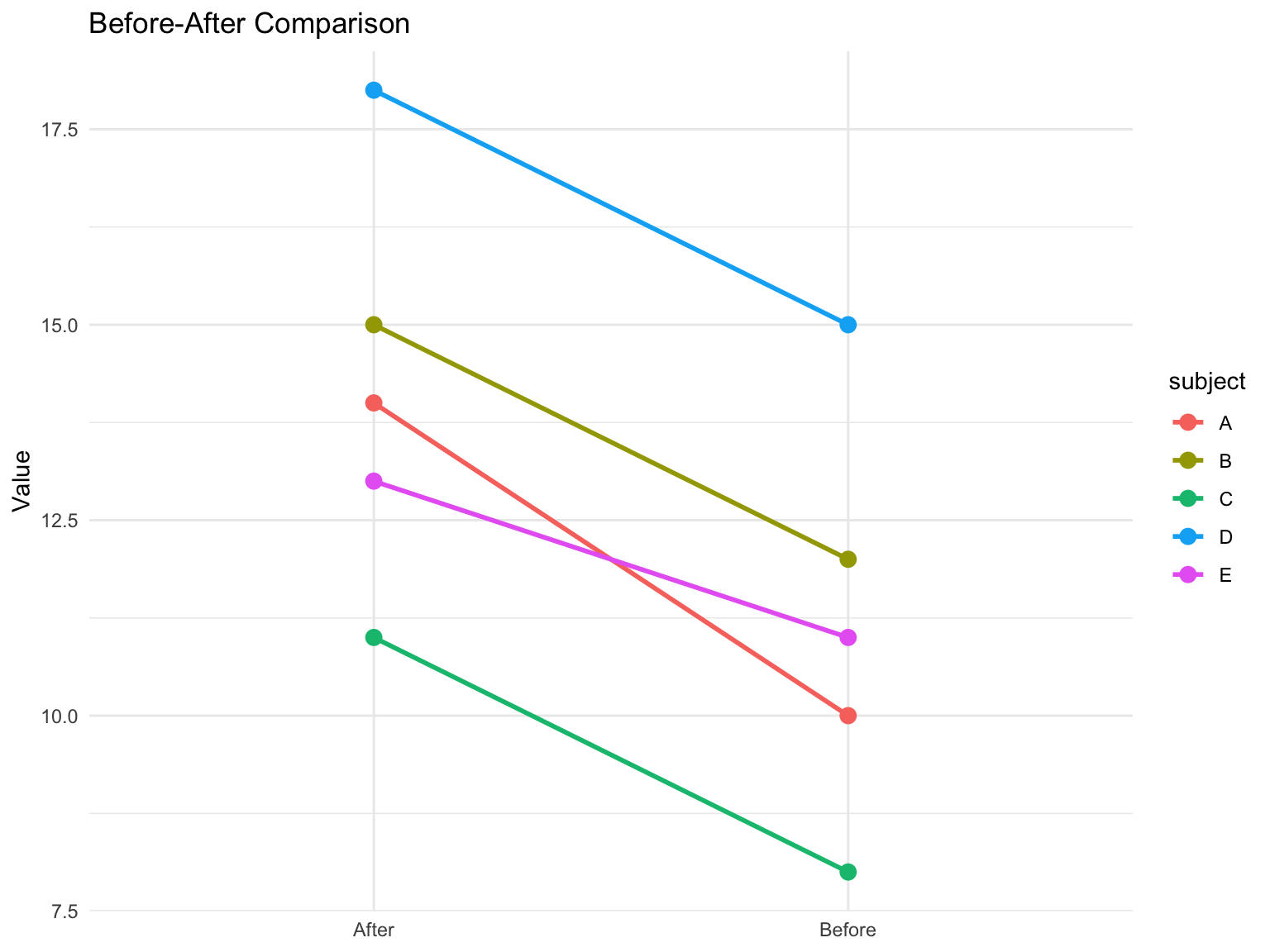
Slope charts effectively show changes between two time points:
Figure 13.37: Slope chart showing change over time
Dense Data and Overplotting
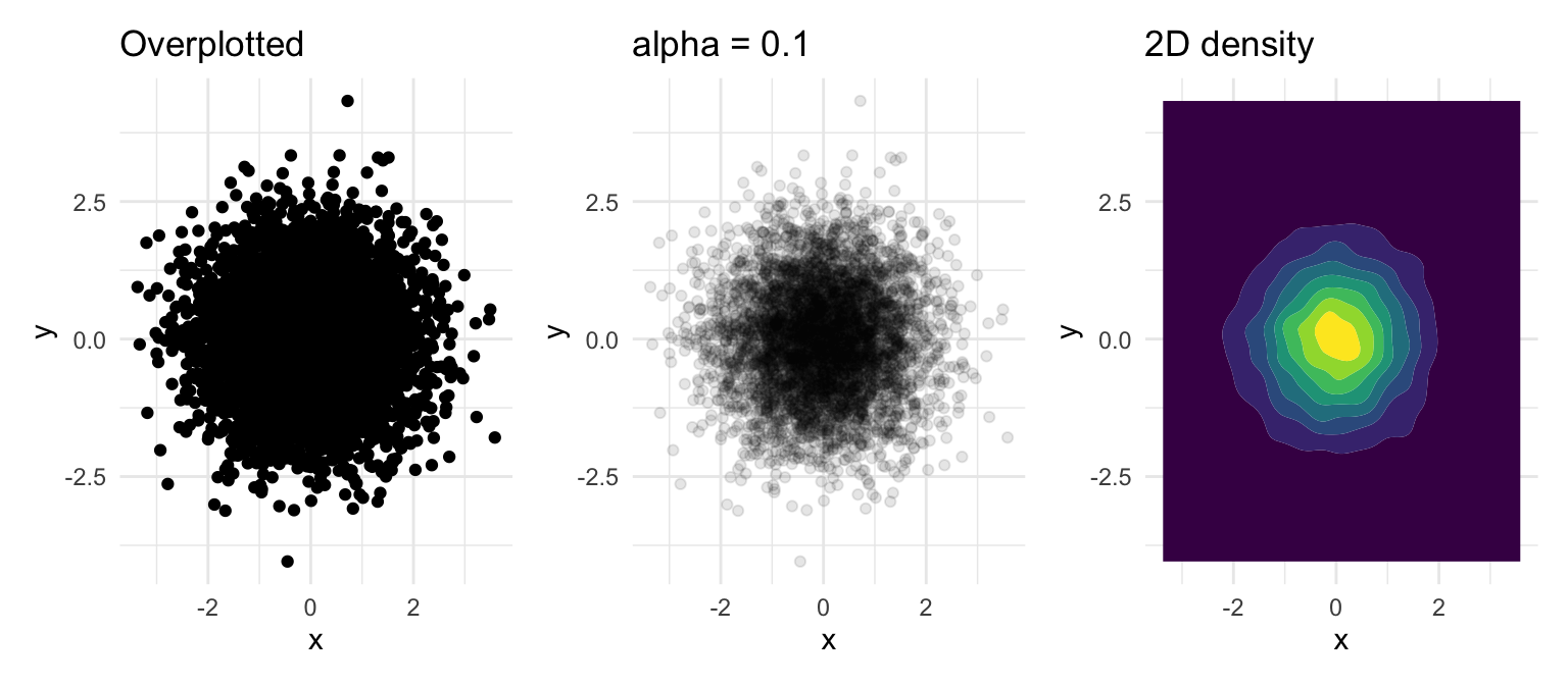
With thousands of observations, a plain scatter plot saturates. Three fixes, in increasing order of summarization: make the points transparent so density shows through, jitter or shrink them, or replace the points with a two-dimensional density estimate that draws the “third dimension” (how many points are here) as filled contours.
Figure 13.38: Five thousand points as opaque dots (left), with alpha = 0.1 (centre), and as filled 2D density contours with geom_density_2d_filled() (right)
geom_hex() and geom_bin_2d() do the same job with hexagonal or square bins and a colour scale for counts, which is often the clearest choice for very large datasets.
13.11 Examples of Poor Graphics
Recognizing bad graphics is the fastest way to learn not to make them. Each of the following breaks one of the principles above.
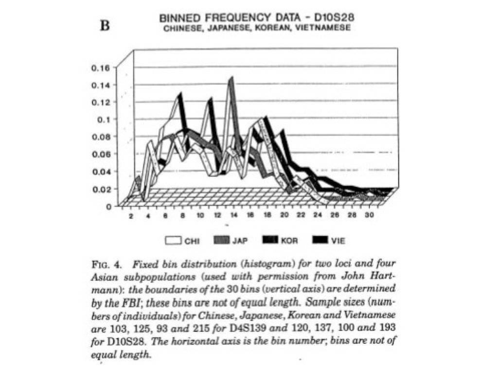
Figure 13.39: A “ticker tape” of unrelated values plotted side by side. There is no question this chart answers: the categories have no order, the lines imply a trend that does not exist, and the reader cannot compare anything.
Figure 13.40: A line to no understanding: lines connect points that are not sequential observations, so the slopes between them mean nothing.
Figure 13.41: A bake sale of pie charts. Comparing angles within one pie is hard; comparing angles across many pies is nearly impossible. A single faceted bar chart or dot plot would show every comparison at once.
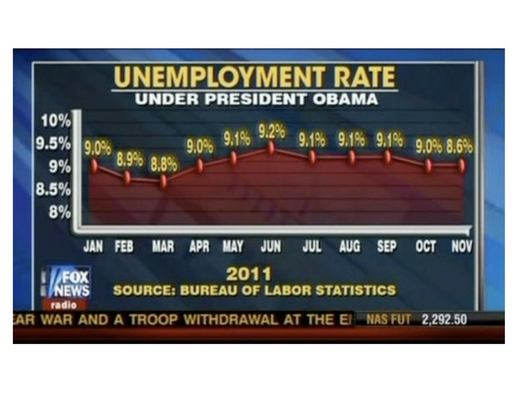
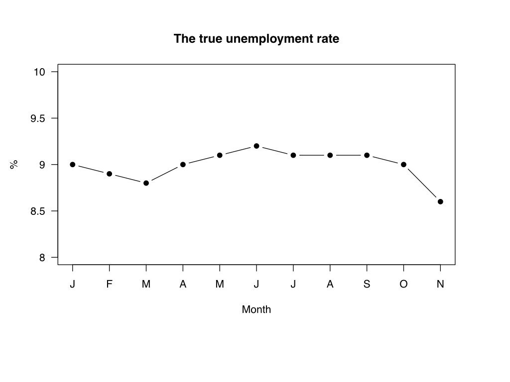
Truncated axes are the most common way a graphic misrepresents magnitudes. Figure 13.42 shows a widely circulated example: a television news graphic of the US unemployment rate whose y-axis started well above zero, so that a change of about one percentage point filled the whole chart, alongside the same data plotted honestly.
(a) As broadcast: the y-axis range is chosen so a small change looks enormous
(b) The same data with an honest axis
Figure 13.42: A truncated y-axis (left) and the honest version (right). Source: Fox News, 2011; Bureau of Labor Statistics data.
“Graphical excellence begins with telling the truth about the data” (Tufte, 1983).
13.12 A Famous Good Example
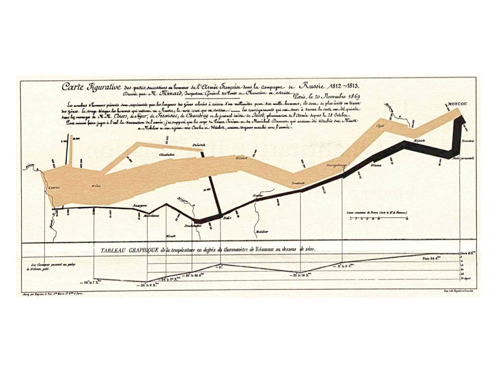
Charles Joseph Minard’s 1869 map of Napoleon’s Russian campaign (Figure 13.43) is often cited as the best statistical graphic ever drawn. It displays six variables in a single coherent image: the size of the army (the width of the band), its position (latitude and longitude), the direction of movement (tan for the advance, black for the retreat), the temperature during the retreat (the line graph beneath), and the date.
Figure 13.43: Minard’s 1869 map of Napoleon’s Russian campaign. Source: Charles Joseph Minard, 1869.
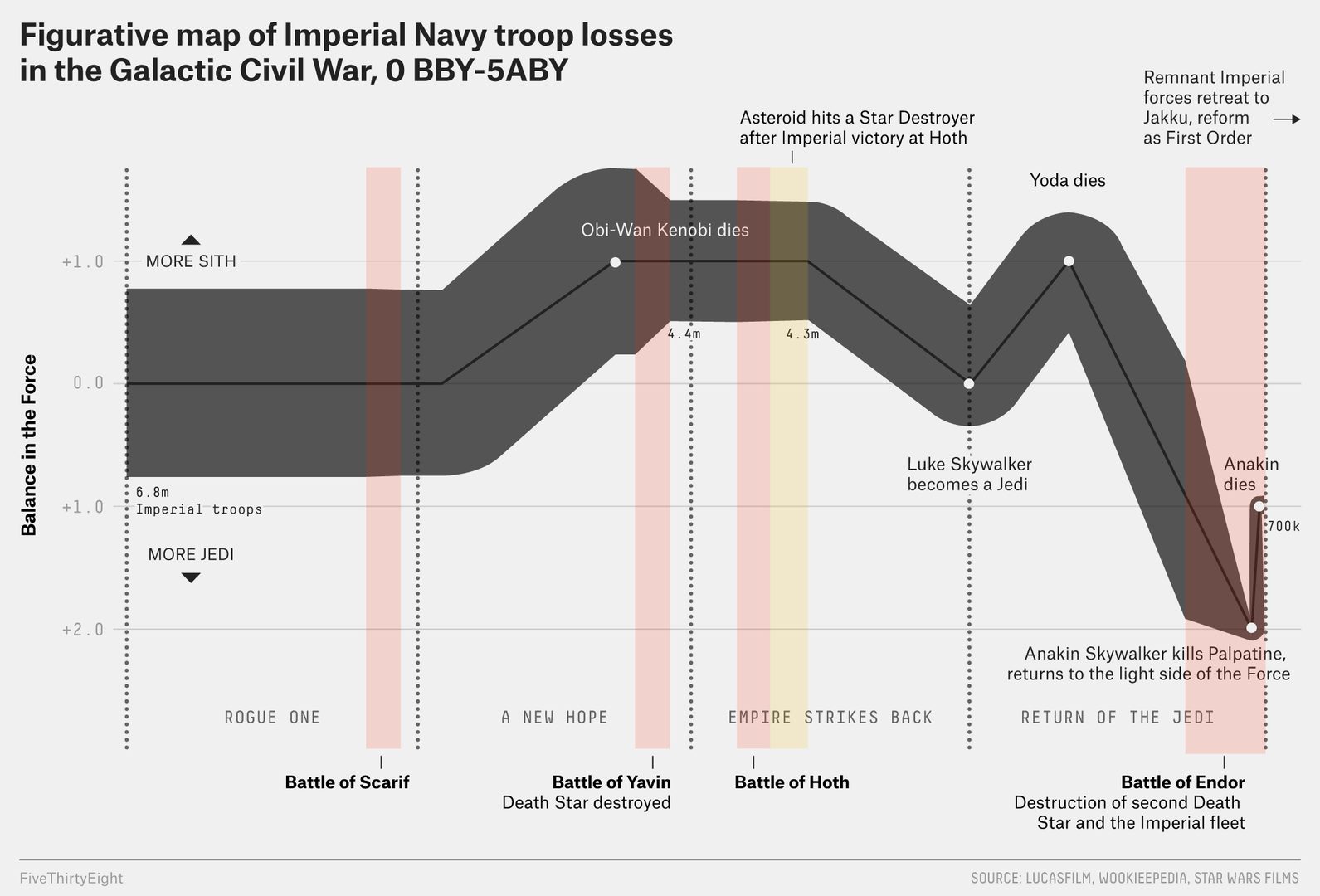
The graphic tells a story without a legend: the army shrinks as it advances, the retreat is devastating, and the losses track the plummeting temperature. Every one of Tufte’s principles is present—the data are shown, the eye is invited to compare the advance with the retreat, magnitudes are honest, there is no clutter, and the meaning is immediate. The same design has been reused for modern data (Figure 13.44), which shows that the idea is a general one: encode the most important quantity as position and width, and let secondary variables ride along as colour and annotation.
Figure 13.44: A modern recreation of Minard’s design applied to a different dataset. Source: FiveThirtyEight.
13.13 Saving Plots
Use ggsave() to export plots; in a Quarto document, figures are instead saved automatically at render time (Section 16.4.5):
# Create a plotp <-ggplot(mtcars, aes(x = wt, y = mpg)) +geom_point() +theme_minimal()# Save as PNG (good for web)ggsave("my_plot.png", plot = p, width =8, height =6, dpi =300)# Save as PDF (good for publications)ggsave("my_plot.pdf", plot = p, width =8, height =6)# Save as SVG (good for editing)ggsave("my_plot.svg", plot = p, width =8, height =6)
ggsave() infers the format from the file extension and, if plot is omitted, saves the last plot displayed. Always give explicit width and height (in inches by default) so that text and points are sized consistently between runs, and use dpi = 300 or higher for raster formats destined for print. Vector formats (PDF, SVG) scale without loss and are what journals usually ask for.
13.14 Running Example: The Stickleback Data
NoteRunning example
This section applies the chapter to the course dataset described in Section 1.5 (80 stickleback, 4 treatment groups, 600 genes). The same steps appear on the Week 6 slides, so the book and the lecture can be read side by side.
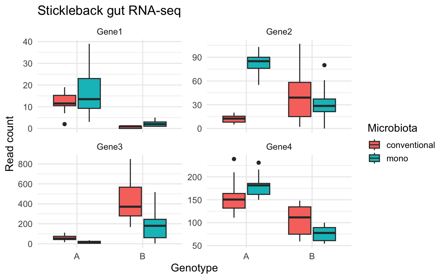
The base R boxplot in Chapter 11 showed one gene. With the long-format data from Chapter 14, ggplot2 shows several genes in one figure: a boxplot layer, colour for the microbiota treatment, and facet_wrap() to give each gene its own panel with its own y-axis.
stickle_long |>filter(gene %in%c("Gene1", "Gene2", "Gene3", "Gene4")) |>ggplot(aes(x = Genotype, y = count, fill = Microbiota)) +geom_boxplot() +facet_wrap(~ gene, scales ="free_y") +labs(y ="Read count", title ="Stickleback gut RNA-seq") +theme_minimal(base_size =14)
Figure 13.45: Read counts for four genes by host genotype and microbiota treatment. Each panel is one gene; colour is the microbiota treatment.
Nothing in the plotting code refers to a particular gene: change the filter() and the same figure describes any subset of the 600. That separation between the data and the description of the graphic is what the grammar of graphics buys you.
13.15 A Gallery of Scientific Figures
The geoms in this chapter cover most day-to-day figures, but bioengineering data regularly calls for a handful of specialized forms. This gallery shows six of them — what question each answers, and the complete code. The first two extend the stickleback running example above; the rest use small synthesized datasets so you can see the data-generating process alongside the figure (the generating code is itself a review of Chapter 11’s random-draw functions).
Figure
The question it answers
Violin + jittered points
what does the whole distribution look like, by group?
Mean–variance plot
how does spread scale with level across many variables?
Clustered heatmap + dendrograms
which samples and which variables behave alike?
Time course with ribbons
how do trajectories differ, and how noisy are they?
Dose–response curve
where is the IC50?
PCA scores plot
what structures a high-dimensional dataset?
Violins and Jittered Points
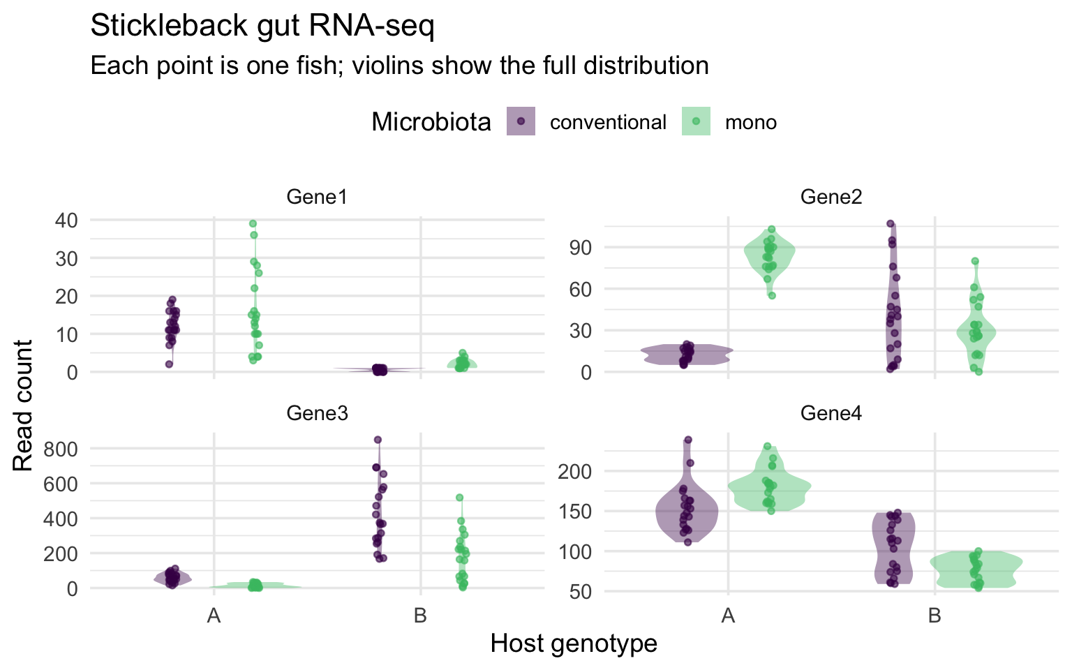
A boxplot summarizes a distribution with five numbers, which can hide bimodality and makes small groups look more certain than they are. Showing the full distribution as a violin, with the raw observations jittered on top, keeps both the summary and the evidence in view:
stickle_long |>filter(gene %in%c("Gene1", "Gene2", "Gene3", "Gene4")) |>ggplot(aes(Genotype, count, fill = Microbiota)) +geom_violin(alpha =0.4, color =NA, position =position_dodge(0.8)) +geom_point(aes(color = Microbiota), alpha =0.6, size =1.2,position =position_jitterdodge(jitter.width =0.08, dodge.width =0.8)) +scale_fill_viridis_d(end =0.7) +scale_color_viridis_d(end =0.7) +facet_wrap(~ gene, scales ="free_y") +labs(x ="Host genotype", y ="Read count",title ="Stickleback gut RNA-seq",subtitle ="Each point is one fish; violins show the full distribution") +theme_minimal(base_size =14) +theme(legend.position ="top")
Figure 13.46: The running example upgraded: violins show each group’s full distribution, and every fish is visible as a point. position_jitterdodge() separates the two microbiota groups and spreads the points sideways.
This is the “show the data” principle from Section 13.9.1 taken to its conclusion: the summary (violin) and every observation coexist in one figure. In Python, sns.violinplot() plus sns.stripplot() build the same figure.
The Mean–Variance Relationship
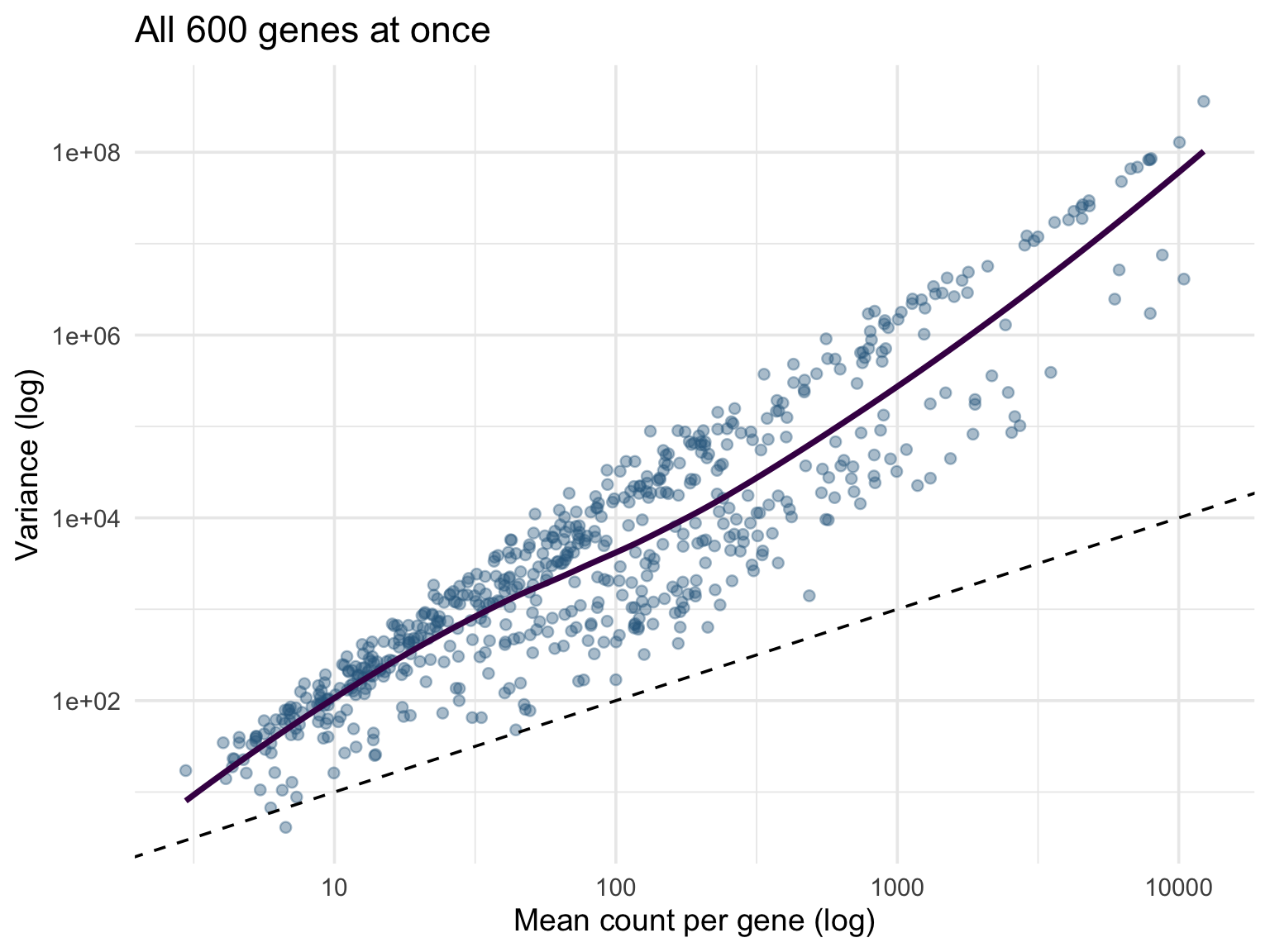
With hundreds of variables measured on the same scale — genes, metabolites, sensor channels — one of the most informative first figures plots each variable’s variance against its mean, on log scales. For count data it answers a specific statistical question: a Poisson process would put every point on the line variance = mean, so points above the line reveal overdispersion:
stickle_long |>group_by(gene) |>summarize(mean =mean(count), var =var(count)) |>ggplot(aes(mean, var)) +geom_point(alpha =0.4, color ="#31688e") +geom_abline(slope =1, intercept =0, linetype ="dashed") +geom_smooth(se =FALSE, color ="#440154") +scale_x_log10() +scale_y_log10() +labs(x ="Mean count per gene (log)", y ="Variance (log)",title ="All 600 genes at once") +theme_minimal(base_size =14)
Figure 13.47: Mean versus variance for all 600 stickleback genes, on log scales. The dashed line marks variance = mean (the Poisson expectation); essentially every gene sits above it, which is why RNA-seq analysis uses the negative binomial distribution.
Note what made this one-liner possible: the long format. group_by(gene) collapses 48,000 rows to 600 — one point per gene — with no loops and no column bookkeeping.
Clustered Heatmaps and Dendrograms
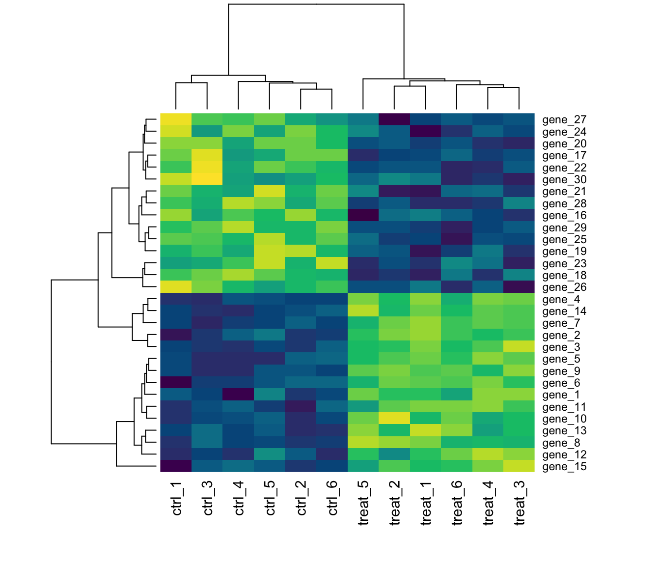
A heatmap displays a whole matrix as color, and hierarchical clustering reorders its rows and columns so that similar ones sit together; the dendrograms on the margins record the clustering tree. Base R’s heatmap() does all of this in one call. Here we synthesize an expression matrix with two gene modules and a control/treated split, then check that the clustering rediscovers the structure we built in:
set.seed(2026)expr <-matrix(rnorm(30*12, mean =8, sd =0.4), nrow =30) +rnorm(30) # a baseline level per geneexpr[1:15, 7:12] <- expr[1:15, 7:12] +2# module 1: up in treatedexpr[16:30, 7:12] <- expr[16:30, 7:12] -1.5# module 2: down in treatedrownames(expr) <-paste0("gene_", 1:30)colnames(expr) <-c(paste0("ctrl_", 1:6), paste0("treat_", 1:6))heatmap(expr, scale ="row", col =hcl.colors(50, "viridis"), margins =c(6, 5))
Figure 13.48: A synthesized 30-gene × 12-sample expression matrix, row-standardized and clustered. The column dendrogram separates control from treated samples, and the row dendrogram recovers the two gene modules.
scale = "row" standardizes each gene before coloring, so the heatmap compares patterns across samples rather than absolute expression levels — without it, the highest-expressed genes would dominate the color range. For publication heatmaps with annotation bars and finer control, see the pheatmap and ComplexHeatmap packages; in Python, seaborn.clustermap() is the equivalent one-liner.
Time Courses with Ribbons
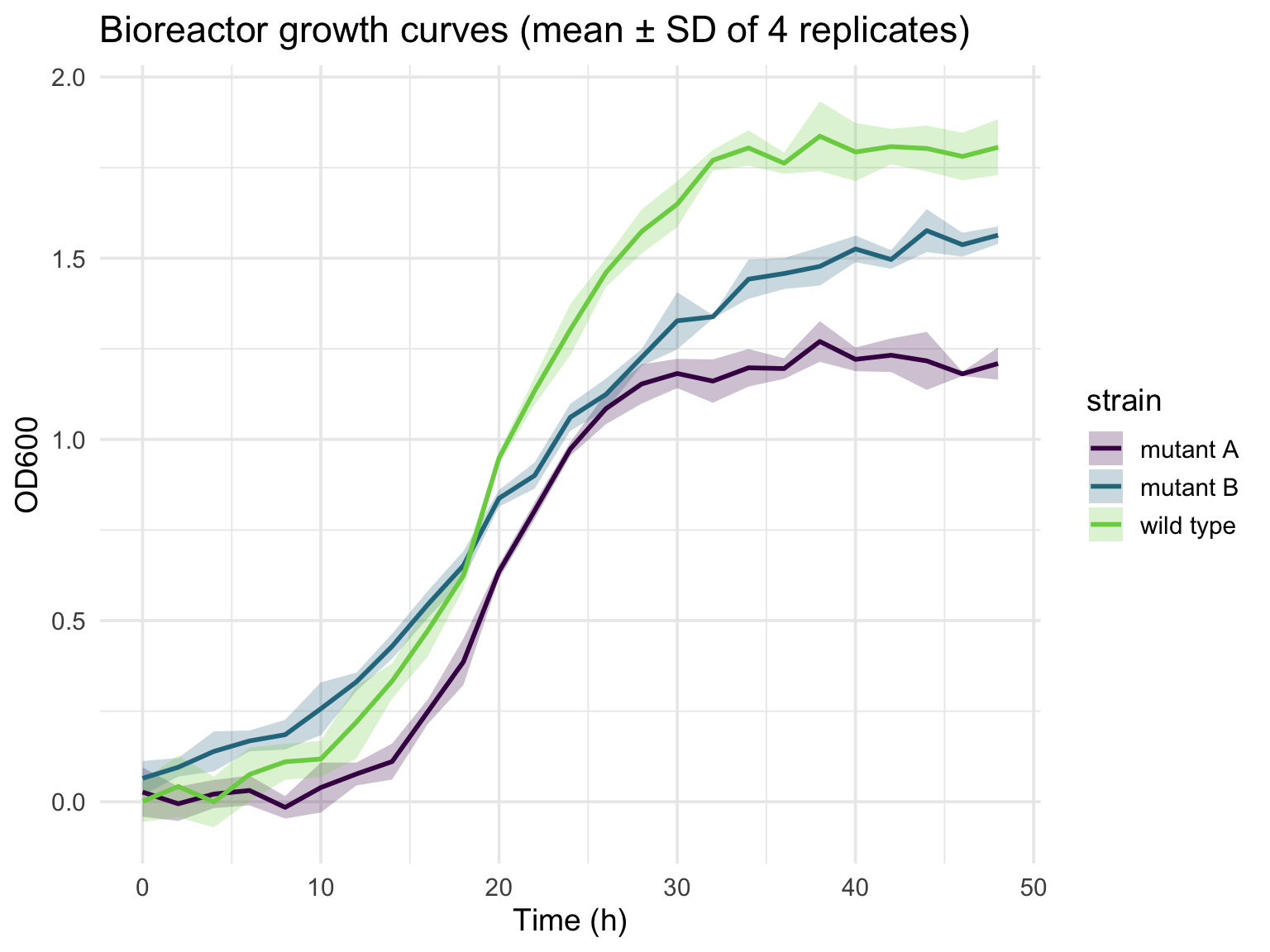
Repeated measurements over time — bioreactor sensors, growth curves, cyclic mechanical loading — are best shown as a mean trajectory per group with a ribbon for the variation. The pattern is always the same: summarize to mean and SD per group per time point, then layer geom_ribbon() under geom_line():
params <-tibble(strain =c("wild type", "mutant A", "mutant B"),K =c(1.8, 1.2, 1.6), # carrying capacityr =c(0.25, 0.35, 0.15)) # growth rategrowth <-expand_grid(params, rep =1:4, time =seq(0, 48, by =2)) |>mutate(od = K / (1+exp(-r * (time -20))) +rnorm(n(), sd =0.05))growth |>group_by(strain, time) |>summarize(mean =mean(od), sd =sd(od), .groups ="drop") |>ggplot(aes(time, mean, color = strain, fill = strain)) +geom_ribbon(aes(ymin = mean - sd, ymax = mean + sd), alpha =0.25, color =NA) +geom_line(linewidth =1) +scale_color_viridis_d(end =0.8) +scale_fill_viridis_d(end =0.8) +labs(x ="Time (h)", y ="OD600",title ="Bioreactor growth curves (mean ± SD of 4 replicates)") +theme_minimal(base_size =14)
Figure 13.49: Synthesized bioreactor growth: three strains following logistic curves with different capacities and rates, measured in quadruplicate with noise. Lines are replicate means; ribbons span ± one SD.
In Python, plt.fill_between(t, mean - sd, mean + sd) draws the ribbon.
Dose–Response Curves
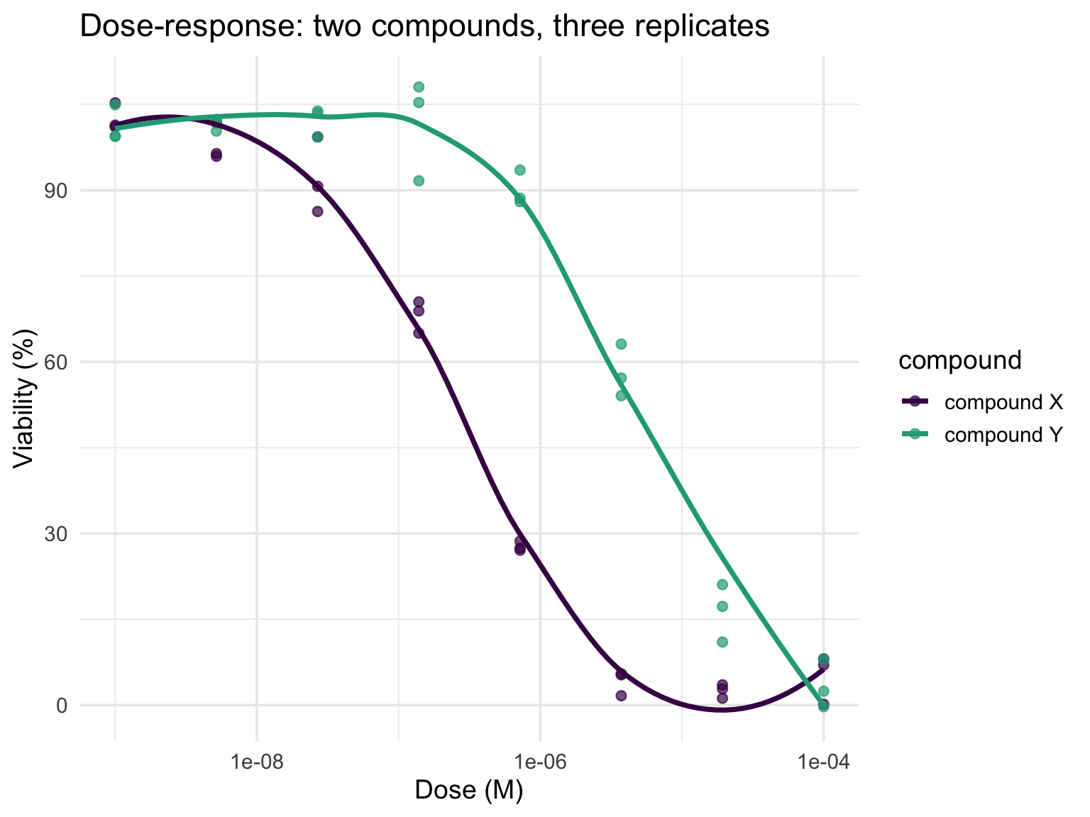
Doses in a response assay span orders of magnitude, so the x-axis must be logarithmic (Section 13.8.3) or all the action collapses against the axis. Points carry the replicates; a smooth line carries the trend; the IC50 is read off where a curve crosses 50%:
dr <-expand_grid(tibble(compound =c("compound X", "compound Y"),ic50 =c(3e-7, 5e-6)),rep =1:3,dose =10^seq(-9, -4, length.out =8)) |>mutate(viability =100/ (1+ (dose / ic50)^1.2) +rnorm(n(), sd =4))ggplot(dr, aes(dose, viability, color = compound)) +geom_point(alpha =0.7, size =2) +geom_smooth(se =FALSE) +scale_x_log10() +scale_color_viridis_d(end =0.6) +labs(x ="Dose (M)", y ="Viability (%)",title ="Dose-response: two compounds, three replicates") +theme_minimal(base_size =14)
Figure 13.50: Synthesized viability data for two compounds (three replicates each) generated from logistic curves with IC50s of 0.3 µM and 5 µM. The log-scaled x-axis is what makes the sigmoids visible.
geom_smooth() draws a data-driven trend, which is fine for exploration; a real potency analysis fits a four-parameter logistic model (the drc package) so that the IC50 comes with a confidence interval.
PCA Scores Plots
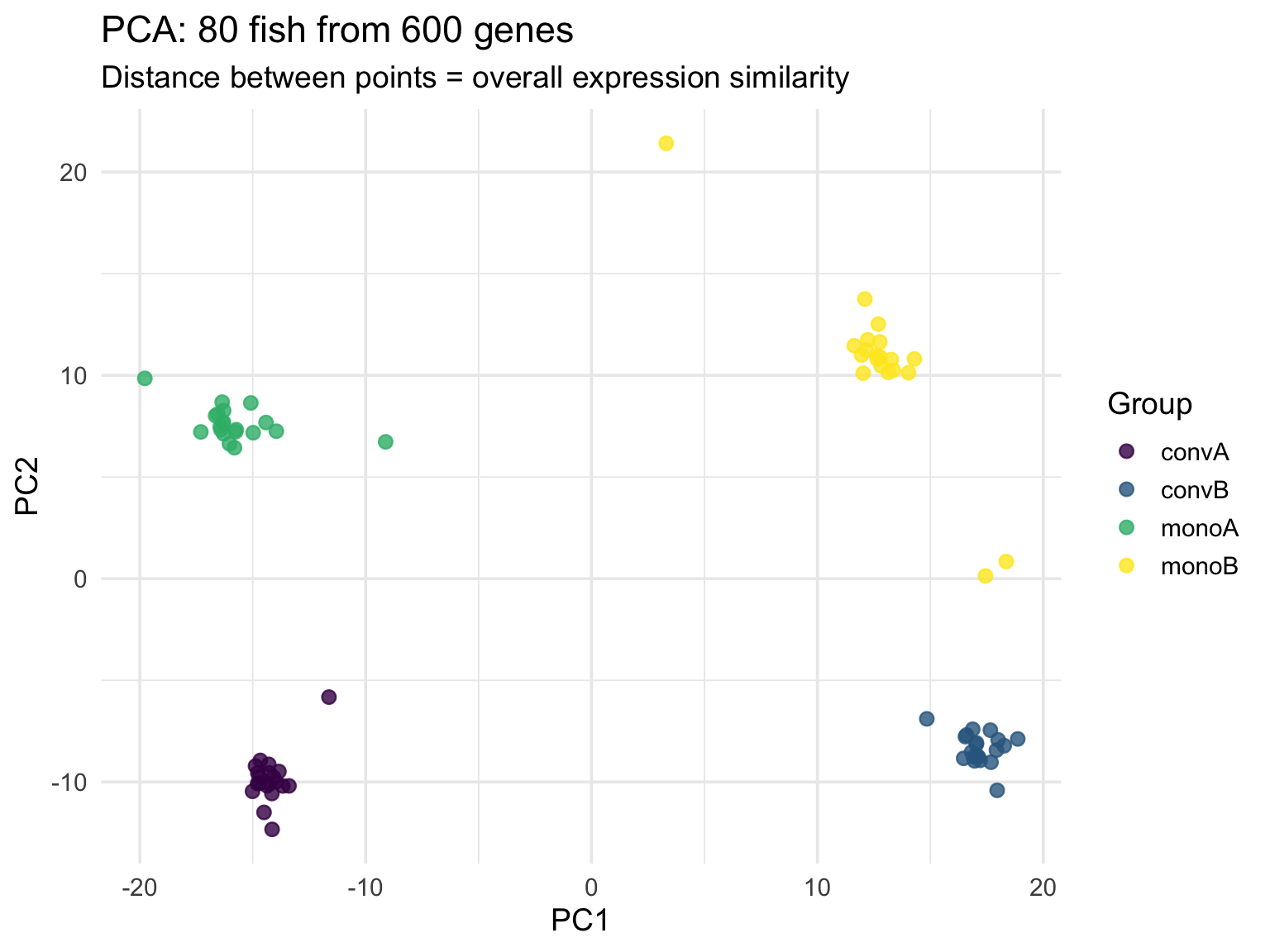
Principal component analysis compresses many correlated columns into a few axes of maximal variation, and plotting the first two components is the standard first look at any high-dimensional dataset. Applied to the real stickleback matrix — 80 fish described by 600 genes — two lines of analysis and one ggplot call reveal the experimental structure:
stickle_wide <-read_tsv("../data/Stickle_RNAseq.tsv", show_col_types =FALSE)pca <-prcomp(log1p(stickle_wide |>select(starts_with("Gene"))), scale. =TRUE)bind_cols(as_tibble(pca$x[, 1:2]), stickle_wide |>select(group =`Geno&Micro`)) |>ggplot(aes(PC1, PC2, color = group)) +geom_point(size =2.5, alpha =0.8) +scale_color_viridis_d(name ="Group") +labs(title ="PCA: 80 fish from 600 genes",subtitle ="Distance between points = overall expression similarity") +theme_minimal(base_size =14)
Figure 13.51: The 80 stickleback placed by the first two principal components of their 600 log-transformed gene counts, colored by genotype-by-microbiota group. Distance between points reflects overall expression similarity.
log1p() (log of 1 + x) tames the right-skewed counts while handling zeros, and scale. = TRUE gives every gene equal weight regardless of its expression level. The summary(pca) output reports how much variance each component captures. In Python, sklearn.decomposition.PCA plays the role of prcomp().
13.16 Summary
ggplot2 provides a powerful and consistent framework for data visualization:
Build plots layer by layer using the Grammar of Graphics
Map data to aesthetics (x, y, color, size, shape) inside aes(); set constants outside it
Add geometries to represent data visually
Use faceting to create multi-panel figures (small multiples)
Reach for the specialized forms when the question calls for them: violins, mean-variance plots, clustered heatmaps, ribbons, dose-response curves, PCA (Section 13.15)
Customize with themes, theme() tweaks, labels, log scales, and color scales matched to the variable type (qualitative, sequential, diverging)
Best practices for effective visualization:
Show the data when possible
Use position and length over angles and area; avoid pie charts
Order categories meaningfully
Include zero for bar charts; show the natural range for line and scatter plots
Use colorblind-friendly palettes and redundant encodings (colour plus shape)
Avoid chart junk, 3D effects, dual y-axes, and rainbow scales
Use transparency or 2D density for dense data
Save with explicit dimensions, and prefer vector formats for publication
Tip
For a reference of ggplot2 functions and R visualization commands, see Appendix E.
ggpubr Package — Publication-ready plots with statistical annotations
Exercises
TipPractice Exercises
Exercise 1: Basic Scatter Plot
Using the iris dataset: 1. Create a scatter plot of Sepal.Length vs Sepal.Width 2. Color points by Species 3. Add appropriate labels and a title
Exercise 2: Distribution Visualization
Using the diamonds dataset: 1. Create a histogram of carat 2. Experiment with different bin widths 3. Add a density curve overlay
Exercise 3: Grouped Comparisons
Using mtcars: 1. Create box plots of mpg grouped by cyl 2. Add jittered points to show individual observations 3. Use a colorblind-friendly palette
Exercise 4: Faceted Plot
Using the diamonds dataset: 1. Create a scatter plot of carat vs price 2. Facet by cut 3. Add a smoothed trend line to each panel
Exercise 5: Publication-Ready Figure
Create a polished figure using any dataset that includes: 1. Meaningful title and axis labels 2. A clean theme 3. Appropriate colors 4. No chart junk 5. Save it as a high-resolution PNG
Exercise 6: Mapped vs. Set
Plot hwy against displ from mpg with aes(color = "blue") inside aes() and explain what you see
Fix it so all points are blue
Map class to colour and drv to shape in one plot; then facet by drv instead and decide which is easier to read
Exercise 7: Scales and Honesty
Plot price against carat for diamonds with and without scale_x_log10() and scale_y_log10(); which reveals the relationship?
Make a bar chart of mean hwy by class and truncate the y-axis with coord_cartesian(); then repeat with ylim() and explain why the two differ
Find a chart in a news article or paper that violates one of the principles in Section 13.9, name the violation, and sketch (in ggplot2) how you would fix it
Anscombe, F. J. (1973). Graphs in statistical analysis.
Cleveland, W. S., & McGill, R. (1984). Graphical perception: Theory, experimentation, and application to the development of graphical methods.
Tufte, E. R. (1983). The visual display of quantitative information.