12 Python Programming Fundamentals
After completing this chapter, you will be able to:
- Install Python 3 on your laptop and load it on Talapas, and explain why every project gets its own virtual environment
- Run Python code from the REPL, from a script, from a Jupyter notebook, and from a
{python}chunk in Quarto - Work with Python’s basic types, strings and f-strings, and its core collections (lists, tuples, dictionaries, sets)
- Use NumPy arrays for vectorized numerical work
- Write control flow, functions with defaults, docstrings and type hints, and handle errors with
try/except - Read and write text and CSV files with
pathlib,open(), andcsv - Load, filter, transform, group, merge, and sort tabular data with pandas
- Make plots with matplotlib and seaborn
- Write command-line scripts that take arguments with
sys.argvandargparse - Translate between R idioms and their Python equivalents
12.1 Why Python, Too?
Chapter 11 introduced R, the language this book uses for statistics, tidy data, and graphics. Python is the other language you will meet constantly in bioengineering. It is a general-purpose language created by Guido van Rossum in 1991, and over the past fifteen years it has become the default language for machine learning, image analysis, instrument control, and much of bioinformatics tooling. If a colleague in an engineering lab hands you code, it is more likely to be Python than R.
The good news is that almost everything you learned in R transfers. Variables, vectors, data frames, functions, loops, reading files, and plotting all exist in Python under slightly different names, and this chapter is organized to follow Chapter 11 section by section so you can map one onto the other. The chapter ends with a translation table (Table 12.7) that you can keep open while you work.
As in Chapter 11, we use a small gene-expression experiment (five samples, two drugs, one response measurement) and a handful of DNA sequences whose GC content we compute. Every section reuses these so that you can concentrate on the syntax rather than the data.
Like R, Python is an interpreted language: you type an expression and see the result immediately. Unlike R, Python was not designed for statistics, so numerical arrays (NumPy), data frames (pandas), and plotting (matplotlib, seaborn) all live in add-on packages that you install and import. Base Python is small and general; the scientific stack sits on top of it.
12.2 Installing Python
There are several ways to get Python 3, and in Chapter 2 you probably already used the first. Which one you choose matters less than using one of them consistently.
python.org installer. Download from https://www.python.org/downloads/. On Windows, check “Add python.exe to PATH” during installation. This gives you a single system-wide Python plus pip, the package installer.
uv. A fast, modern tool from Astral that installs Python versions, creates environments, and installs packages, all with one command-line program. Install it once, then uv python install 3.12 fetches an interpreter. It is the quickest route on macOS and Linux.
conda (Miniconda or Miniforge). A package manager that installs Python and non-Python software (samtools, R, compilers) into isolated environments. It is heavier than venv but is the standard on HPC systems and in bioinformatics. Choose the Miniforge installer: it defaults to the free community conda-forge channel, whereas Anaconda’s default channel requires a paid license at organizations like UO.
On Talapas. Nothing to install: use the module system described in Chapter 20.
Check whichever installation you have:
python vs python3
On many systems python is either missing or points to an old Python 2. Always type python3 at the shell (and #!/usr/bin/env python3 in scripts) unless you are inside an activated environment, where python is safe. On Windows outside WSL the launcher is py.
12.3 Virtual Environments
R users install packages once into a library and load them with library(). Python users go one step further: each project gets its own virtual environment, a private folder holding a copy of the interpreter’s links and every package the project needs. This prevents the situation where upgrading pandas for one analysis silently breaks another. Section 2.10 introduced the idea; here is the full workflow.
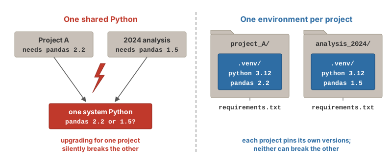
.venv with pinned versions, recorded in a requirements.txt that anyone can rebuild from.
# Create an environment in the project folder (do this once)
python3 -m venv .venv

# Activate it (every time you open a new terminal)
source .venv/bin/activate          # macOS, Linux, WSL
# .venv\Scripts\activate           # Windows PowerShell

# Install packages into it
pip install numpy pandas matplotlib seaborn

# Record exactly what is installed, for reproducibility
pip freeze > requirements.txt

# Later, on another machine:
pip install -r requirements.txt

# Leave the environment
deactivate
With uv the same steps are shorter and much faster:
With conda, environments live in a central location rather than in the project folder, and can include non-Python tools:
Unlike venv, conda environments are named and central rather than per-folder—conda env list shows them all—and packages come from community channels (conda-forge for general software, bioconda for genomics tools). mamba, included in Miniforge, is a faster drop-in replacement for the conda command.
R has the same idea in the renv package: renv::init() run once inside a project creates a private package library, renv::snapshot() records the exact versions in a renv.lock file, and renv::restore() rebuilds the library from that file on any machine (its use on Talapas is shown in Chapter 20). Table 12.1 compares the three tools.
| Tool | For | Environments live… | The record you share |
|---|---|---|---|
venv (+ pip) |
Python | in the project folder (.venv/) |
requirements.txt |
conda / mamba
|
Python plus compiled tools (samtools, even R) |
centrally, by name (conda env list) |
environment.yml |
renv |
R | in the project folder | renv.lock |
Whichever tool you use, the rule is the same: commit the record file to Git, never the environment itself.
Add .venv/ to your .gitignore (Chapter 19). Commit requirements.txt or environment.yml instead; anyone can rebuild the environment from that file.
12.4 Running Python Code
Python offers the same console-versus-script choice as R, plus notebooks.
The REPL. Type python3 at the shell to get the interactive prompt (>>>). Type an expression, see the result, and exit() when done. In Positron and VS Code, the Python console is the same thing with a nicer interface.
Scripts. Save code in a .py file and run it with python3 script.py. To make it directly executable, add a shebang and set the permission bit, exactly as for a shell script (Chapter 10):
Jupyter notebooks. pip install jupyter then jupyter lab opens a browser-based notebook in which code cells and Markdown cells alternate and outputs are saved in the .ipynb file. Notebooks are excellent for exploration and are what you will get on Talapas through Open OnDemand.
Quarto chunks. In a .qmd file a {python} chunk runs through Jupyter when the document renders (Chapter 16):
In this chapter the Python chunks are shown with their expected output as trailing # comments rather than executed at render time, so that the book builds on a machine with R alone.
12.5 Python Basics: Types, Arithmetic, and Variables
Arithmetic
Note that ^ is not exponentiation in Python (it is bitwise XOR), and that the mathematical functions live in the math module.
Variables and Assignment
Assignment uses =; there is no <-. Names follow the same rules as R (letters, digits, underscores; case-sensitive; cannot start with a digit), and the convention is snake_case.
Basic Types
Table 12.2 lists the basic types with their R equivalents (compare Table 11.2).
| Python type | Description | Example | R equivalent |
|---|---|---|---|
int |
Integer (arbitrary size) | 42 |
integer (42L) |
float |
Real number | 3.14 |
numeric |
str |
Text string | "gene1" |
character |
bool |
Logical |
True, False
|
logical (TRUE, FALSE) |
None |
Absence of a value | None |
NULL (and, loosely, NA) |
Comparisons and Logical Operators
Comparison operators are the same as R. Logical operators are spelled out as words:
5 > 3                # True
5 == 5               # True
5 != 3               # True

True and False       # False   (R: &&)
True or False        # True    (R: ||)
not True             # False   (R: !)

"TP53" in ["BRCA1", "TP53", "EGFR"]   # True    (R: %in%)

# Floating point is the same everywhere
0.1 + 0.2 == 0.3                       # False
math.isclose(0.1 + 0.2, 0.3)           # True    (R: all.equal / near)
Getting Help
Python’s counterpart of R’s ?mean (Section 11.8.4) is help(), which prints a function’s docstring (Section 12.10). In IPython (Pérez & Granger, 2007), Jupyter, and Positron’s Python console, a trailing ? gives the short version and ?? adds the source code:
import numpy as np
import inspect

help(np.mean)                 # full documentation, works in any Python
np.mean?                      # short help - IPython, Jupyter, Positron only
np.mean??                     # ...plus the source code

dir(np)                                 # everything a module (or object) contains
[n for n in dir(np) if "mean" in n]     # like apropos("mean") in R
inspect.signature(np.mean)              # like args(mean) in R
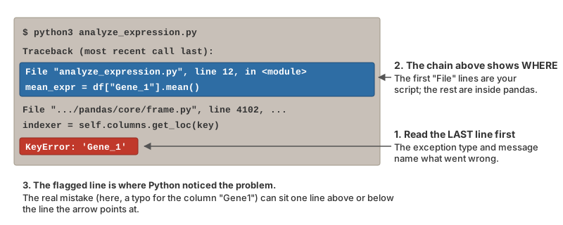
The official references are excellent and worth bookmarking: https://docs.python.org/3/ for the language and standard library, https://numpy.org/doc/ and https://pandas.pydata.org/docs/ for the scientific stack. As in R, when an error message defeats you, search the exact text—and read tracebacks from the bottom up (Section 12.15).
12.6 Strings and f-strings
Strings are first-class in Python and carry many methods. Indexing is 0-based, and slicing s[start:stop] excludes stop.
seq = "ATGCGCGATATCG"

len(seq)             # 13
seq[0]               # 'A'      first character (R: substr(seq, 1, 1))
seq[-1]              # 'G'      last character
seq[0:3]             # 'ATG'    characters 0, 1, 2
seq[3:]              # 'CGCGATATCG'

seq.count("G")       # 4
seq.lower()          # 'atgcgcgatatcg'
seq.replace("T", "U")            # 'AUGCGCGAUAUCG'
seq.startswith("ATG")            # True
"gene,sample,value".split(",")   # ['gene', 'sample', 'value']
"_".join(["S1", "control"])      # 'S1_control'
"  padded  ".strip()             # 'padded'
f-strings put values inside text with {} and optional format specifications. They replace paste()/sprintf() from R:
12.7 Lists, Tuples, Dictionaries, and Sets
Python’s built-in containers do the work of R’s vectors and lists, but note that a Python list is more like an R list() than like a vector: it can hold mixed types, and arithmetic does not apply element-wise (that is NumPy’s job, Section 12.8). Table 12.3 compares the four containers.
| Container | Syntax | Mutable? | Ordered? | Use for |
|---|---|---|---|---|
list |
[1, 2, 3] |
Yes | Yes | Ordered collections you will change |
tuple |
(1, 2, 3) |
No | Yes | Fixed records, multiple return values |
dict |
{"a": 1} |
Yes | Yes (insertion) | Key-value lookups (R: named list) |
set |
{1, 2, 3} |
Yes | No | Unique values, membership, set algebra |
Lists
measurements = [2, 3, 4, 2, 1, 2, 4, 5, 10, 8, 9]
samples = ["control", "treatment_A", "treatment_B"]

measurements[0]          # 2        (R: measurements[1])
measurements[-1]         # 9        last element
measurements[1:4]        # [3, 4, 2]
len(measurements)        # 11

samples.append("treatment_C")     # add to end (modifies in place)
samples.sort()                    # sorts in place
sorted(measurements, reverse=True)   # returns a new sorted list

sum(measurements)        # 50
max(measurements)        # 10
measurements.index(10) # 8 position of the value 10y = x does not copy a list (or a NumPy array, or a pandas DataFrame): it gives the same object a second name, so a change made through either name is visible through both. Ask for a copy explicitly when you want one.
R behaves differently—y <- x acts like a copy, because R copies objects when they are modified—which is exactly why this surprise bites R users hardest.
A list comprehension applies an expression to every element, taking the place of sapply()/purrr::map() and of many for loops:
Tuples
Dictionaries
A dictionary maps keys to values and is the closest thing to an R named list or named vector:
expression = {"BRCA1": 5.2, "TP53": 8.1, "EGFR": 3.4}

expression["TP53"]               # 8.1
expression["KRAS"] = 9.7         # add a key
"EGFR" in expression             # True
expression.get("MYC", 0.0)       # 0.0  default when key is missing

list(expression.keys())          # ['BRCA1', 'TP53', 'EGFR', 'KRAS']
list(expression.values())        # [5.2, 8.1, 3.4, 9.7]

for gene, value in expression.items():
    print(f"{gene}: {value}")
# BRCA1: 5.2
# TP53: 8.1
# ...
Sets
12.8 NumPy Arrays
NumPy provides the n-dimensional array, the object that makes Python behave like R’s vectors and matrices: same-type elements, element-wise arithmetic, and fast numerical routines. Import it as np by convention.
import numpy as np

x = np.array([2, 3, 4, 2, 1, 2, 4, 5, 10, 8, 9])

x * 2                    # array([ 4,  6,  8,  4,  2,  4,  8, 10, 20, 16, 18])
x ** 2                   # element-wise square
np.log(x)                # element-wise log
x + np.arange(1, 12)     # element-wise addition of two arrays

x.mean(), x.std(ddof=1)  # (4.545..., 3.110...)   ddof=1 gives R's sample sd
np.median(x)             # 4.0
x[x > 5]                 # array([10,  8,  9])   logical indexing, as in R
np.where(x > 5)          # (array([8, 9, 10]),)  (R: which(x > 5), but 0-based)

# Sequences (R: seq, rep)
np.arange(0, 10, 0.5)              # 0, 0.5, ..., 9.5
np.linspace(0, 1, 5)               # array([0.  , 0.25, 0.5 , 0.75, 1.  ])
np.repeat(["A", "B"], 3)           # ['A','A','A','B','B','B']

# Matrices (R: matrix)
mat = np.arange(1, 13).reshape(3, 4)
mat.shape                # (3, 4)
mat[0, 1]                # 2      row 0, column 1
mat[:, 2]                # third column
mat.T                    # transpose
mat.sum(axis=0)          # column sums (R: apply(mat, 2, sum))
mat.sum(axis=1) # row sums (R: apply(mat, 1, sum))Missing values in NumPy are np.nan (a float), and like R’s NA they propagate unless you ask for the NaN-aware versions:
12.9 Control Flow
Python uses indentation instead of braces to mark blocks. Four spaces per level is the universal convention; a colon ends the line that opens a block.
score = 85

if score >= 90:
    grade = "A"
elif score >= 80:
    grade = "B"
else:
    grade = "C"
grade                    # 'B'

# for loops iterate directly over any collection
for sample in ["S1", "S2", "S3"]:
    print(sample)

# range() gives integer sequences (0-based, stop excluded)
for i in range(5):
    print(i ** 2)        # 0 1 4 9 16

# enumerate() gives index and value together
for i, gene in enumerate(["BRCA1", "TP53"]):
    print(i, gene)       # 0 BRCA1 / 1 TP53

# zip() walks two sequences in parallel (R: mapply / map2)
for gene, value in zip(["BRCA1", "TP53"], [5.2, 8.1]):
    print(f"{gene}={value}")

# while loops, break and continue as in bash and R
n = 0
while n < 3:
    n += 1
    if n == 2:
        continue
    print(n)             # 1 3
A vectorized conditional (R’s ifelse()) is np.where():
12.10 Functions
Functions are defined with def. The body is indented, and return sends a value back; a function with no return returns None. Defaults, keyword arguments, and positional matching work as in R.
def gc_content(seq, digits=3):
    """Return the GC fraction of a DNA sequence.

    Parameters
    ----------
    seq : str
        DNA sequence (case-insensitive).
    digits : int, optional
        Number of decimal places to round to.
    """
    seq = seq.upper()
    gc = seq.count("G") + seq.count("C")
    return round(gc / len(seq), digits)

gc_content("ATGCGCGATATCG")             # 0.538
gc_content("atgcgc", digits=1)          # 0.7
gc_content(digits=2, seq="GGCC")        # 1.0   named arguments in any order
The triple-quoted string right after def is the docstring, Python’s built-in documentation. help(gc_content) prints it, exactly as ?mean does in R, and IDEs show it on hover. Write one for every function you expect to reuse (Chapter 15 covers function design in R; the same principles apply).
Type hints annotate the expected types. Python does not enforce them, but editors and AI assistants (Chapter 18) use them to catch mistakes and to complete your code:
Small anonymous functions use lambda, the equivalent of R’s \(x):
12.11 Reading and Writing Files
pathlib.Path represents file paths portably; open() opens a file and the with block closes it automatically when you are done.
from pathlib import Path

data_dir = Path("data")
fasta = data_dir / "sequences.fasta"     # / joins path components
fasta.exists()                           # True
fasta.suffix                             # '.fasta'
list(data_dir.glob("*.csv"))             # all CSV files in data/

# Read a whole file as one string, or line by line
text = fasta.read_text()

with open(fasta) as fh:
    n_records = sum(1 for line in fh if line.startswith(">"))
print(n_records)                         # 3

# Write text
Path("results.txt").write_text(f"{n_records} records\n")

with open("log.txt", "a") as fh:         # "a" appends; "w" overwrites
    fh.write("finished\n")
A minimal FASTA parser using only built-ins:
def read_fasta(path):
    """Return a dict mapping sequence names to sequences."""
    seqs = {}
    name = None
    with open(path) as fh:
        for line in fh:
            line = line.strip()
            if line.startswith(">"):
                name = line[1:].split()[0]
                seqs[name] = ""
            elif name:
                seqs[name] += line
    return seqs

for name, seq in read_fasta("data/sequences.fasta").items():
    print(f"{name}\t{len(seq)}\t{gc_content(seq)}")
# seq1    60    0.483
# seq2    72    0.611
# seq3    45    0.400
The csv module handles quoting and delimiters for you when you need row-by-row access; for anything tabular, though, pandas (Section 12.12) is easier.
12.12 pandas DataFrames
pandas is Python’s data-frame library, and its DataFrame plays the role of R’s data.frame/tibble. If you know dplyr (Section 14.3), you already know what each method does; Table 12.4 lists the correspondences.
Creating and Inspecting
import pandas as pd

experiment = pd.DataFrame({
    "sample_id":     ["S1", "S2", "S3", "S4", "S5"],
    "treatment":     ["control", "drug_A", "drug_A", "drug_B", "drug_B"],
    "concentration": [0, 10, 20, 10, 20],
    "response":      [1.2, 3.4, 5.6, 2.8, 4.1],
})

experiment
#   sample_id treatment  concentration  response
# 0        S1   control              0       1.2
# 1        S2    drug_A             10       3.4
# 2        S3    drug_A             20       5.6
# 3        S4    drug_B             10       2.8
# 4        S5    drug_B             20       4.1

experiment.shape           # (5, 4)        (R: dim)
experiment.columns         # Index(['sample_id', ...])   (R: names)
experiment.dtypes          # column types  (R: str)
experiment.head(3)         # first rows
experiment.describe()      # summary statistics (R: summary)
experiment.info()          # structure overview
Reading and Writing
df = pd.read_csv("data/experiment.csv")                 # R: read.csv / read_csv
df = pd.read_csv("data/counts.tsv", sep="\t")           # tab-separated
df = pd.read_csv("data.csv", na_values=["", "NA", "N/A"])
df = pd.read_excel("data.xlsx")                          # needs openpyxl

experiment.to_csv("results.csv", index=False)            # index=False drops the row numbers
experiment.to_csv("results.tsv", sep="\t", index=False)
Selecting and Filtering
experiment["response"]                     # one column -> Series (R: df$response)
experiment[["sample_id", "response"]]      # several columns -> DataFrame
experiment.loc[0]                          # row by label
experiment.iloc[0:3]                       # rows by position (0-based)
experiment.loc[0:2, ["treatment", "response"]]

# Filtering rows (R: filter / df[df$response > 3, ])
experiment[experiment["response"] > 3]
experiment.query("treatment == 'drug_A' and response > 3")
experiment[experiment["treatment"].isin(["drug_A", "drug_B"])]
Adding Columns, Sorting, Grouping
# mutate: add or transform columns (assign returns a new frame)
experiment = experiment.assign(
    log_response = np.log(experiment["response"]),
    replicate    = [1, 1, 2, 1, 2],
)
experiment["high"] = experiment["response"] > 3         # or assign directly

# arrange
experiment.sort_values("response", ascending=False)
experiment.sort_values(["treatment", "response"])

# group_by + summarise
experiment.groupby("treatment")["response"].mean()
# treatment
# control    1.20
# drug_A     4.50
# drug_B     3.45

experiment.groupby("treatment").agg(
    n            = ("response", "size"),
    mean_resp    = ("response", "mean"),
    sd_resp      = ("response", "std"),
).reset_index()
#   treatment  n  mean_resp   sd_resp
# 0   control  1       1.20       NaN
# 1    drug_A  2       4.50  1.555635
# 2    drug_B  2       3.45  0.919239

# count
experiment["treatment"].value_counts()
Merging and Chaining
doses = pd.DataFrame({
    "treatment": ["control", "drug_A", "drug_B"],
    "target":    ["none", "EGFR", "BRAF"],
})

merged = experiment.merge(doses, on="treatment", how="left")    # R: left_join

# Method chaining is the pandas equivalent of the pipe |>
summary = (
    experiment
    .query("concentration > 0")
    .assign(log_response=lambda d: np.log(d["response"]))
    .groupby("treatment", as_index=False)
    .agg(mean_log=("log_response", "mean"))
    .sort_values("mean_log", ascending=False)
)
Table 12.4 translates the dplyr verbs of Section 14.3 into pandas.
| dplyr | pandas |
|---|---|
filter(df, x > 3) |
df[df["x"] > 3] or df.query("x > 3")
|
select(df, a, b) |
df[["a", "b"]] |
mutate(df, y = x * 2) |
df.assign(y=df["x"] * 2) or df["y"] = df["x"] * 2
|
arrange(df, x) / arrange(df, desc(x))
|
df.sort_values("x") / df.sort_values("x", ascending=False)
|
group_by(df, g) \|> summarise(m = mean(x)) |
df.groupby("g")["x"].mean() or .agg(m=("x", "mean"))
|
count(df, g) |
df["g"].value_counts() or df.groupby("g").size()
|
rename(df, new = old) |
df.rename(columns={"old": "new"}) |
distinct(df, g) |
df["g"].unique() or df.drop_duplicates("g")
|
left_join(a, b, by = "k") |
a.merge(b, on="k", how="left") |
pivot_longer() / pivot_wider()
|
df.melt() / df.pivot()
|
drop_na(df) |
df.dropna() |
df \|> f() \|> g() |
df.f().g() (method chaining) |
Missing values in pandas are NaN (or pd.NA), and df.isna(), df.dropna(), and df.fillna(0) correspond to is.na(), drop_na(), and replace_na().
A column that should be numeric but arrived as text—because of a stray entry such as "n/a" or "<1"—is converted with pd.to_numeric(). Plain float("n/a") raises a ValueError, but errors="coerce" turns unconvertible entries into NaN instead, the pandas counterpart of as.numeric() returning NA with a warning in R (Section 11.7):
12.13 Plotting with matplotlib and seaborn
matplotlib is the foundational plotting library, analogous to base R graphics; seaborn sits on top of it with data-frame-aware, statistically minded functions that feel closer to ggplot2. If you love ggplot2, the plotnine package is a faithful port of the grammar of graphics to Python (from plotnine import ggplot, aes, geom_point) and is worth a look.
import matplotlib.pyplot as plt

x = np.arange(1, 11)
y = x ** 2

fig, ax = plt.subplots(figsize=(6, 4))
ax.scatter(x, y, color="darkblue")
ax.set_title("Quadratic Relationship")
ax.set_xlabel("X values")
ax.set_ylabel("Y values")
fig.savefig("quadratic.png", dpi=150)     # R: png(); plot(); dev.off()
plt.show()Overlaying the theoretical density on that histogram takes one more package: scipy.stats (pip install scipy) provides distribution objects whose methods mirror R’s four-letter families (Section 11.17.1). Where R has rnorm(), dnorm(), pnorm(), and qnorm(), Python splits the jobs between the NumPy generator (random draws) and scipy.stats (everything else), as Table 12.5 shows.
scipy.stats offers the same methods for uniform, poisson, binom, and many more
| Job | R | Python |
|---|---|---|
| Random draws | rnorm(n, 0, 1) |
rng.normal(0, 1, n) or norm.rvs(size=n)
|
| Density at x | dnorm(x) |
norm.pdf(x) |
| Cumulative probability P(X ≤ x) | pnorm(x) |
norm.cdf(x) |
| Quantile | qnorm(p) |
norm.ppf(p) |
Every ax. call draws onto the same figure until plt.show()—matplotlib’s version of R’s curve(..., add = TRUE) (Section 11.17). To place several panels in one figure, ask plt.subplots() for a grid of axes and draw on each one, the counterpart of par(mfrow = c(2, 2)) (Section 11.14.5):
seaborn works directly from a DataFrame, with x=, y=, and hue= playing the part of aes():
import seaborn as sns

sns.set_theme(style="whitegrid")

fig, ax = plt.subplots(figsize=(5, 4))
sns.boxplot(data=experiment, x="treatment", y="response", ax=ax)
sns.stripplot(data=experiment, x="treatment", y="response",
              color="black", size=6, ax=ax)
ax.set_ylabel("Response")
plt.show()

# Multi-panel figures (R: facet_wrap) come from relplot / catplot
sns.relplot(data=experiment, x="concentration", y="response",
            col="treatment", kind="scatter")
Many further plot types follow the same pattern: sns.histplot, sns.violinplot, sns.lineplot, sns.heatmap, and sns.pairplot. Chapter 13 explains the design principles that apply whichever library you use.
12.14 Command-Line Scripts
A Python script becomes a reusable tool once it reads its inputs from the command line, exactly as a shell script uses $1 (Section 10.7) and an R script uses commandArgs() (Section 10.10). The simplest approach is sys.argv, a list whose first element is the script name:
For anything with options, argparse builds the parser, generates --help, and validates types:
#!/usr/bin/env python3
# gc_stats.py - GC content for every record in a FASTA file
import argparse
from pathlib import Path

parser = argparse.ArgumentParser(description="GC content per FASTA record")
parser.add_argument("fasta", type=Path, help="input FASTA file")
parser.add_argument("-o", "--output", type=Path, default=None,
                    help="write a TSV here instead of stdout")
parser.add_argument("--min-length", type=int, default=0,
                    help="skip sequences shorter than this")
args = parser.parse_args()

rows = [(name, len(seq), gc_content(seq))
        for name, seq in read_fasta(args.fasta).items()
        if len(seq) >= args.min_length]

out = "\n".join(f"{n}\t{l}\t{g}" for n, l, g in rows) + "\n"
if args.output:
    args.output.write_text(out)
else:
print(out, end="")The idiom if __name__ == "__main__": at the bottom of a script lets the same file be both imported as a module (to reuse gc_content() elsewhere) and run as a program. Scripts like these are exactly what you submit to Slurm on Talapas (Chapter 20) inside a shell wrapper.
12.15 Error Handling
Python raises exceptions when something goes wrong; a try/except block catches them so that your script can report a clear message or recover, the counterpart of R’s tryCatch() (see also Section 21.7 for purrr’s safely()).
try:
    df = pd.read_csv("data/missing.csv")
except FileNotFoundError:
    print("Input file not found; check the path")

# Catch several, and always run cleanup
try:
    value = float("abc")
except (ValueError, TypeError) as err:
    print(f"Could not convert: {err}")
finally:
    print("done")
# Could not convert: could not convert string to float: 'abc'
# done

# Raise your own errors when inputs are invalid (R: stop())
def gc_content_checked(seq):
    if not seq:
        raise ValueError("sequence is empty")
    return gc_content(seq)
Common exceptions you will meet: FileNotFoundError, KeyError (missing dictionary key or column), IndexError (position out of range), TypeError, ValueError, and ZeroDivisionError. Reading the last line of a traceback tells you which one occurred; the lines above it show where.
Table 12.6 collects the messages you will meet most often, with their usual cause and fix—the counterpart of the R table in Table 11.4.
| Error message | Meaning | Fix |
|---|---|---|
NameError: name 'x' is not defined |
No variable with that name exists | Check spelling and case; run the cell or lines that create it |
ModuleNotFoundError: No module named 'pandas' |
The package is not installed in this environment | Activate the right environment, pip install it, check which python3 or the IDE’s interpreter picker |
SyntaxError / IndentationError
|
Missing : or bracket, or inconsistent indentation |
Look at the line above the arrow too; use four spaces, never tabs |
TypeError: unsupported operand type(s) |
Arithmetic on the wrong type (e.g., a string) | Check with type() or df.dtypes; convert explicitly |
KeyError: 'Gene1' |
Dictionary key or DataFrame column does not exist | Check spelling; print df.columns or d.keys()
|
IndexError: list index out of range |
Position past the end (remember 0-based indexing) | Check len(x); the last element is x[-1]
|
ValueError: could not convert string to float |
A value has the right type but an invalid content | Inspect the offending value; for columns, pd.to_numeric(col, errors="coerce")
|
FileNotFoundError |
Wrong path or working directory | Check Path.cwd(); use project-relative paths |
... continuation prompt in the REPL |
Python is waiting for you to finish an expression | Close the open bracket or quote (or press Ctrl-C) |
Figure 12.2 shows how to read the traceback that accompanies these messages.
12.16 R and Python Side by Side
Table 12.7 gathers the correspondences from this chapter in one place.
| Concept | R | Python |
|---|---|---|
| Assignment | x <- 5 |
x = 5 |
| Indexing | 1-based: x[1] is first |
0-based: x[0] is first; x[-1] is last
|
| Exclude by index |
x[-1] drops the first |
x[1:] |
| Exponent | 2^3 |
2**3 |
| Integer division, modulo |
%/%, %%
|
//, %
|
| Vector | c(1, 2, 3) |
[1, 2, 3] (list) or np.array([1, 2, 3])
|
| Named list / lookup | list(a = 1, b = 2) |
{"a": 1, "b": 2} (dict) |
| Sequence |
1:10, seq(0, 1, 0.1)
|
range(1, 11), np.arange(0, 1.1, 0.1)
|
| Logical operators |
&, \|, !, %in%
|
and, or, not, in (scalars); &, \|, ~ on arrays |
| Missing values |
NA, NULL, NaN
|
None, np.nan, pd.NA
|
| Ignore missing | mean(x, na.rm = TRUE) |
np.nanmean(x), df["x"].mean() (skips NaN) |
| String concatenation |
paste0(a, b), sprintf()
|
a + b, f"{a}{b}"
|
| Tabular data |
data.frame(), tibble |
pd.DataFrame() |
| Read CSV |
read.csv(), read_csv()
|
pd.read_csv() |
| Column access | df$col |
df["col"] |
| dplyr verbs |
filter, select, mutate, arrange, group_by/summarise
|
query/boolean mask, [[...]], assign, sort_values, groupby/agg
|
| Joins | left_join(a, b, by = "k") |
a.merge(b, on="k", how="left") |
| Pipeline | df \|> f() \|> g() |
df.f().g() |
| Apply over elements |
sapply(x, f), purrr::map(x, f)
|
[f(v) for v in x] |
| Vectorized if | ifelse(cond, a, b) |
np.where(cond, a, b) |
| Define function | f <- function(x, n = 2) { ... } |
def f(x, n=2): ... |
| Anonymous function | \(x) x^2 |
lambda x: x**2 |
| Help | ?mean |
help(np.mean), docstrings |
| Load package | library(dplyr) |
import pandas as pd |
| Install package | install.packages("dplyr") |
pip install pandas (or uv pip, conda) |
| Project isolation | renv |
venv, uv, conda |
| Script arguments | commandArgs(trailingOnly = TRUE) |
sys.argv[1:], argparse
|
| Error handling |
tryCatch(), stop()
|
try/except, raise
|
| Random seed | set.seed(42) |
np.random.default_rng(42) |
| Plots | base graphics, ggplot2 | matplotlib, seaborn, plotnine |
| Notebook document |
.qmd with {r}
|
.qmd with {python}, or .ipynb
|
You do not have to pick one. Quarto documents can mix {r} and {python} chunks (Chapter 16), the reticulate R package calls Python from R, and Positron (Chapter 2) runs both consoles side by side. A common pattern is to preprocess with Python tools and then model and plot in R, or the reverse. Fluency in the translation table is what makes that painless.
12.17 Running Example: The Stickleback Data
This section applies the chapter to the course dataset described in Section 1.5 (80 stickleback, 4 treatment groups, 600 genes). The same steps appear on the Week 6 slides, so the book and the lecture can be read side by side.
In Python the same steps go through pandas. read_csv() with sep="\t" reads the tab-separated file, .shape and .iloc play the roles of dim() and bracket indexing, and pd.crosstab() is table():
A grouped boxplot is one method call on the data frame, with matplotlib doing the drawing:
The reshaping and grouped summaries that Chapter 14 does with pivot_longer() and group_by() have direct pandas equivalents in melt() and groupby(); Table 12.4 maps each verb to its counterpart.
Here is that reshaping on the stickleback table itself. The awkward column name Geno&Micro is fixed once with rename(), melt() turns the 600 gene columns into a gene/count pair (80 × 600 = 48,000 rows), and a grouped aggregation computes every gene’s mean in every treatment group in one chain:
stickle = stickle.rename(columns={"Geno&Micro": "geno_micro"})   # fix the awkward name once

stickle_long = stickle.melt(
    id_vars=["Individual", "Genotype", "Microbiota", "geno_micro"],
    var_name="gene", value_name="count")
stickle_long.shape                     # (48000, 6): one row per fish x gene

gene_means = (
    stickle_long
    .groupby(["gene", "Genotype", "Microbiota"], as_index=False)
    .agg(mean_count=("count", "mean"))
)
gene_means.query("gene == 'Gene1'")
These are the same four numbers per gene that the tidyverse pipeline produces in Section 14.11, and the comparison is worth making side by side: rename()/rename(columns=), pivot_longer()/melt(), and group_by() |> summarize()/groupby().agg() line up verb for verb.
12.18 Summary
This chapter introduced Python 3 as a second language alongside R:
- Install Python from python.org,
uv, or conda; on Talapas,module load python3 - Every project gets a virtual environment (
python3 -m venv .venv,uv venv, orconda create), andrequirements.txtorenvironment.ymlrecords it - Run code from the REPL,
python3 script.py(with#!/usr/bin/env python3), Jupyter, or{python}chunks in Quarto - Assignment is
=, indexing is 0-based,**is exponentiation, and blocks are marked by indentation - Strings have many methods and f-strings format output; lists, tuples, dicts, and sets are the built-in containers
- NumPy arrays give R-style vectorized arithmetic; remember
ddof=1for the sample standard deviation - Functions use
def, defaults, docstrings, and optional type hints;lambdamakes small anonymous functions -
pathlib,open(), andcsvhandle files; pandas handles tables withread_csv, boolean masks,assign,groupby/agg,merge, andsort_values - matplotlib and seaborn make figures; plotnine ports ggplot2
-
sys.argvandargparseturn scripts into command-line tools;try/excepthandles errors - Table 12.7 maps R idioms onto Python ones
Appendix F collects the commands from this chapter in a quick-reference format.
Exercises
Exercise 1: Environment and Script
- Create a folder
py-practice, make a virtual environment in it, activate it, and installnumpy,pandas,matplotlib, andseaborn - Write
hello.pywith a shebang that prints your name and today’s date (from datetime import date), make it executable, and run it with./hello.py - Run
pip freeze > requirements.txtand look at the file
Exercise 2: Strings and Collections
- Write a function
reverse_complement(seq)that returns the reverse complement of a DNA string (hint: a dictionary mapping bases,reversed(), and"".join()) - Given
genes = ["BRCA1", "TP53", "EGFR", "KRAS", "TP53"], use a set to count the unique genes and a dictionary to count how often each appears - Use a list comprehension to keep only genes whose name starts with a letter before “M”
Exercise 3: NumPy
- Create an array of the integers 1 to 20 and compute the mean, median, and sample standard deviation
- Extract the even numbers with a boolean mask
- Reshape the array into 4 rows by 5 columns and compute the row and column sums
Exercise 4: pandas
Recreate the experiment data frame from Section 12.12, then:
- Filter to rows with
concentration > 0 - Add a
log_responsecolumn - Compute the mean and standard deviation of
responsebytreatment - Save the result as a CSV file and read it back
Exercise 5: A Command-Line Tool
- Write
fasta_stats.pythat takes a FASTA filename fromargparseand prints, for each record, its name, length, and GC content - Add a
--min-gcoption that filters records - Wrap the parsing in
try/exceptso that a missing file gives a friendly message instead of a traceback - Compare your script with the bash version in Section 10.12
Exercise 6: Translation
Take the split-apply-combine example from Section 11.15 (mean mpg by cyl in mtcars) and reproduce it in pandas. The dataset is available from seaborn’s data repository, or export it from R with write.csv(mtcars, "mtcars.csv").
Additional Resources
- The Python Tutorial — The official introduction, concise and authoritative
- Python for Data Analysis — Wes McKinney, the creator of pandas; free online
- NumPy user guide and pandas user guide
- seaborn tutorial and plotnine documentation
- Biopython — Sequence parsing, alignment, and more for bioinformatics
- Scientific Python Lectures — A broader tour of the scientific stack