20 High-Performance Computing with Talapas
After completing this chapter, you will be able to:
- Explain what high-performance computing (HPC) is and when to use it
- Connect to Talapas via SSH, your editor’s Remote-SSH extension, and Open OnDemand
- Navigate the storage system and understand quotas
- Explain how the SLURM scheduler decides which job runs next (fair-share, backfill, QOS limits)
- Write and submit batch jobs using SLURM
- Monitor job status, interpret pending reasons, and right-size requests with
seffandsacct - Use software modules, per-user environments, and containers
- Design a multi-step, multi-sample pipeline that checkpoints, logs, and scales out with job arrays or a workflow manager
- Follow best practices for responsible cluster use
20.1 What is High-Performance Computing?
When your laptop isn’t enough—when analyses run for days, require hundreds of gigabytes of memory, or need specialized hardware like GPUs—you need high-performance computing (HPC).
An HPC cluster is a collection of interconnected computers (called nodes) that work together to solve computational problems. Instead of upgrading your personal computer indefinitely, you submit jobs to a shared resource with far more capability.
When to Use HPC
Consider HPC when:
- Analyses take hours or days on your laptop
- Data is too large to fit in your computer’s memory
- You need GPUs for machine learning
- You want to run many similar jobs in parallel
- Your analysis would monopolize your personal computer
Talapas: UO’s Computing Cluster
Talapas is the University of Oregon’s HPC cluster, named after a Chinook word for coyote (the educator and keeper of knowledge). It’s managed by Research Advanced Computing Services (RACS).
Key resources:
- Over 14,520 CPU cores
- 129 TB of total memory
- 89 GPUs (including NVIDIA A100 and H100)
- 3+ petabytes of storage
20.2 Talapas Architecture
Understanding the cluster architecture (Figure 20.1; compare the generic layout in Figure 4.7) helps you use it effectively.

sbatch or srun, and it runs on CPU, GPU, or high-memory (“fat”) compute nodes that all share the same storage
Login Nodes vs. Compute Nodes
Login nodes are where you:
- Log in and manage files
- Edit scripts
- Submit jobs
- Check job status
Do NOT run computationally intensive work on login nodes! They’re shared by everyone, and heavy processes will be terminated.
Compute nodes are where your actual work runs, accessed through the job scheduler (SLURM) (Yoo et al., 2003).
Node Types
The general-use node types are summarized in Table 20.1.
| Node type (general use) | How many | Cores per node | Memory per node | Purpose |
|---|---|---|---|---|
| Standard CPU (AMD Milan) | 43 | 128 | 512 GB | General computation |
| GPU | 24 | 48 | 256-512 GB | Machine learning, CUDA (52 NVIDIA A100 GPUs in total) |
| Large memory | a few | varies | up to 4 TB | Memory-intensive work (e.g., genome assembly) |
| Interactive | 19 | varies | varies | Testing, development, Open OnDemand sessions |
Across the whole cluster (general-use and condo nodes together) Talapas offers 14,520+ CPU cores, 129 TB of memory, 89 GPUs (A100, H100, and V100), and roughly 3 PB of storage.
Research groups can also purchase condo nodes that their members get priority access to—about 166 additional researcher-owned CPU nodes plus V100, A100, and H100 GPUs. If your lab owns condo nodes, your PI can tell you which partition to use. Numbers here come from RACS Services; check the Talapas Knowledge Base for current counts, since the hardware changes as groups buy in.
Partitions (Queues)
Jobs are submitted to partitions with different characteristics:
| Partition | Time Limit | Use It For |
|---|---|---|
compute |
1 day | Generic CPU jobs (the default choice) |
computelong |
14 days | Long-running CPU jobs |
gpu |
1 day | Jobs that need a GPU |
gpulong |
14 days | Long-running GPU jobs |
interactive |
12 hours | Shorter interactive CPU sessions |
interactivegpu |
8 hours | Shorter interactive GPU sessions |
memory |
1 day | Memory-intensive jobs (up to 4 TB) |
memorylong |
14 days | Long-running, memory-intensive jobs |
Run sinfo on Talapas to see all partitions, including your lab’s condo partitions.
20.3 Getting Access
Step 1: Join a PIRG
Every Talapas user is sponsored by a UO principal investigator and belongs to that PI’s PIRG (Principal Investigator Research Group). The PIRG is both your access group and the account your jobs are charged to. Your PI adds you to an existing PIRG; if your lab does not yet have one, your PI requests a new PIRG by emailing racs@uoregon.edu.
Step 2: Request Access
Access requests go through the Talapas customer portal. You will need your PI’s name and the PIRG you are joining.
Your credentials:
- Username: Your Duck ID
- Password: Your UO password (with Duo two-step verification)
Ask early. Account creation requires your PI to confirm the request, and RACS processes requests during business hours, so allow several days before you need to run anything.
20.4 Connecting to Talapas
Option 1: SSH (Command Line)
From your terminal (macOS Terminal, the Ubuntu (WSL) terminal on Windows, or the terminal in VS Code or Positron):
login.talapas.uoregon.edu is a load balancer that hands you to one of the four login nodes. Expect a Duo two-step prompt after you enter your password: no characters appear while you type the password (this is normal), and Duo then asks you to type 1 for a push notification to the Duo Mobile app, 2 for a text message, or 3 for a phone call. Mac and Linux users can set up an SSH key (ssh-keygen -t ed25519, then ssh-copy-id) to skip the password, but Duo will still prompt whenever policy requires it.
An SSH key is a matched pair of files: a public key (the lock—safe to share, and the thing you hand to servers) and a private key (the key—it never leaves your computer). Give a server your public key once and it recognizes your machine from then on, so you stop typing your password:
ssh-keygen writes the pair to ~/.ssh/: the public half is id_ed25519.pub, the private half id_ed25519 (never share or commit that one). Duo still applies when policy requires it. The same key pair authenticates you to GitHub—Section 19.13.1 shows where to paste the public key there.
Do you need the VPN? The Talapas Knowledge Base says a UO VPN connection is recommended, not required. Without the VPN, connect to the load balancer as above and answer the Duo prompts. With the UO VPN connected, you can also SSH directly to a specific login node:
Connecting to a specific node is useful when you want to reconnect to a tmux or screen session you left running there.
Windows users: Use the Ubuntu (WSL) terminal, or connect from VS Code or Positron with Remote-SSH (Section 20.4.2).
Connecting Your Editor with Remote-SSH
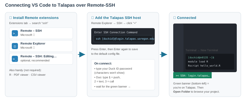
Editing scripts over a bare terminal gets old quickly. Both VS Code and Positron support Remote - SSH, which lets you run your familiar editor on your laptop while the files, terminal, and code execution live on Talapas.
- Install the Remote - SSH extension in VS Code or Positron
- Open the command palette, choose Remote-SSH: Connect to Host…, and enter
yourduckid@login.talapas.uoregon.edu - Enter your UO password and complete the Duo prompt
- Open a folder on Talapas (for example
/projects/myPIRG/yourduckid) and work as usual
The editor’s file browser, search, and integrated terminal now all point at Talapas. Two things to remember:
The integrated terminal in a Remote-SSH session runs on a login node. Use it to edit files, run sbatch and srun, and check squeue, exactly as you would over SSH. Do not run heavy computation in it. If you want an interactive R or Python session with real resources, start an interactive job (Section 20.10) or use Open OnDemand.
A Remote-SSH connection uses SSH under the hood, so the same VPN guidance applies: connecting through login.talapas.uoregon.edu works from anywhere, and the VPN lets you target a specific login node.
Option 2: Open OnDemand (Web Browser)
For a graphical interface with no setup at all, use Open OnDemand at ondemand.talapas.uoregon.edu. Log in with your Duck ID and UO password; a Chrome or Firefox private window avoids login problems caused by cached UO sessions.
Open OnDemand provides:
- Interactive apps: Jupyter Lab, and a remote desktop where you can run RStudio, MATLAB, or Stata with a full graphical interface
- Shell access: a terminal to a login node in your browser tab
- File explorer: browse your home and project directories, and upload and download files by drag-and-drop
- Job composer: build, submit, and monitor SLURM jobs from a form
- Active jobs: see what is running and what is queued
When you launch an interactive app, Open OnDemand submits a SLURM job on your behalf (on the interactive or interactivegpu partition) and connects your browser to it once it starts. Those sessions keep running after you close the browser tab, consuming your allocation until they hit their time limit. When you are done, go back to My Interactive Sessions and delete the session so the resources are released for everyone else.
Open OnDemand is the easiest way to start, and it remains the best option whenever you want a graphical application on cluster hardware.
When Login Fails
Three problems account for almost every failed first connection:
-
Permission denied (publickey,password). Either the password was mistyped or your account is not active yet. Verify that you can sign in to any UO web service with the same Duck ID and password (reset it at duckid.uoregon.edu if needed), then confirm with your PI that the PIRG request went through. If it persists, email RACS. -
The Duo prompt never arrives. Make sure the Duo Mobile app is open and your phone has a network connection. If pushes do not work, type
2at the prompt for a text message or3for a phone call instead of1. -
srun: error: Invalid account or account/partition combination. You submitted a job without--account=<myPIRG>(or with a PIRG you do not belong to). Rungroupsto see which PIRGs you are in, then either add--account=to everysrun/sbatchcall or set it once in your shell profile (see Section 20.6).
20.5 Storage on Talapas
Figure 20.3 shows the layout of the file system, and Table 20.3 lists the quota and purpose of each location.
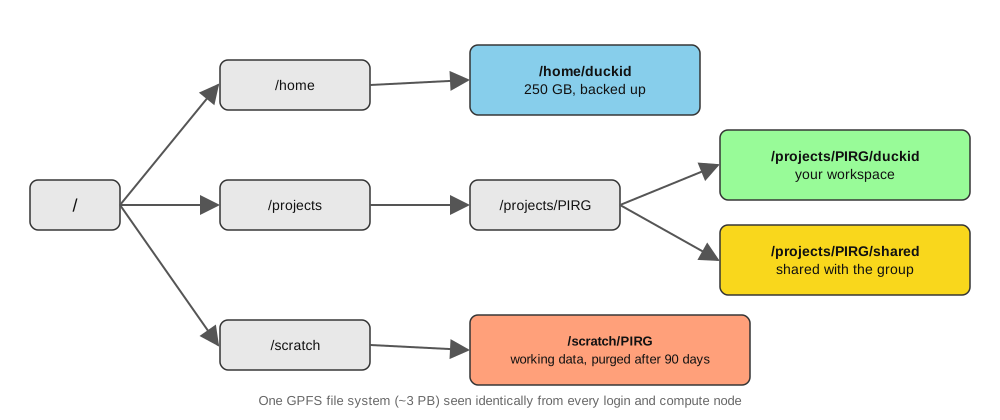
Directory Structure
All of these live on a single ~3 PB parallel file system (IBM GPFS) that looks the same from every login and compute node, so a file you write on the login node is immediately visible to your jobs.
| Location | Quota | Purpose |
|---|---|---|
/home/duckid |
250 GB | Config files, small scripts, per-user software installs |
/projects/PIRG/duckid |
Shared (default 2 TB) | Large data, analysis |
/projects/PIRG/shared |
Shared | Files shared with group |
/scratch/PIRG |
Large per-PIRG quota | High-throughput working space; files untouched for 90 days are purged |
/tmp (on compute nodes) |
Local to node | Temporary scratch space for one job |
Storage Policies
Three policies shape where your files should live:
-
/scratchis purged. Anything in/scratch/<PIRG>/that has not been accessed in 90 days is deleted automatically, without warning. It is the right place for large intermediate files while a pipeline runs (it is fast and has a generous quota), and the wrong place for anything you would miss. When a run finishes, copy the results you want to keep to/projects/<PIRG>/and delete the rest. If/scratch“looks empty after a few months,” this is why. - Nothing is backed up. RACS does not back up any Talapas file system. Some snapshotting exists for home and project directories, but it is not a substitute for your own copies. Keep code in Git (Chapter 19) and irreplaceable data somewhere off the cluster.
-
Home is small and shared. Your home directory is for dotfiles, scripts, and small software installs, not for sequencing data or reference genomes. Put those under
/projects(shared with your lab) or/scratch.
Figure 20.4 condenses these policies into a single decision.
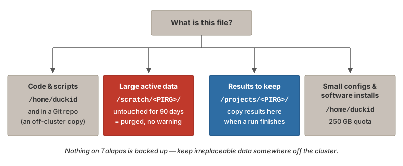
Moving Files On and Off Talapas
For files up to a few gigabytes, scp, rsync, or the Open OnDemand file browser are enough:
# From your laptop: copy a file to your project directory
$ scp results.csv yourduckid@login.talapas.uoregon.edu:/projects/myPIRG/yourduckid/

# Sync a whole directory (only changed files are copied; -a keeps timestamps)
$ rsync -avz data/ yourduckid@login.talapas.uoregon.edu:/projects/myPIRG/yourduckid/data/
For large transfers (tens of gigabytes to terabytes, or thousands of files), RACS recommends Globus. Globus moves data between “endpoints” (Talapas, your laptop with Globus Connect Personal, another university’s cluster, or a cloud bucket) in the background, retries automatically after network interruptions, and verifies checksums on arrival. It is also the tool for moving data to and from UO’s Large-Scale Research Storage (LSRS) for long-term archiving. Log in to Globus with your Duck ID, find the Talapas endpoint, and drag folders between panes; the transfer keeps running after you close the browser.
Check Your Storage
Data is NOT automatically backed up! You are responsible for backing up important files. Consider using Git for code (Chapter 19) and external storage for irreplaceable data (Section 3.4.1).
20.6 SLURM: The Job Scheduler
SLURM (Simple Linux Utility for Resource Management) is the software that manages the cluster (Yoo et al., 2003). It:
- Allocates resources fairly among users
- Queues jobs when resources are busy
- Tracks resource usage
Figure 20.5 traces a job from submission to completion.

sbatch places the job in the queue, it waits for resources, runs on a compute node, and leaves its output in files
Three words recur in everything that follows. A job is a unit of work you submit. A partition is a queue with its own hardware and time limits (Table 20.2). An account is the PIRG your usage is charged to.
SLURM is the dominant scheduler on academic and national-lab clusters worldwide, so everything in this chapter transfers to almost any cluster you will encounter. Its job is to decide when, where, and with what resources every job runs. The mental model is a request-and-grant transaction:
- You declare what your job needs: how many CPU cores, how much memory, how long it will run, and whether it needs a GPU.
- SLURM looks across all the nodes, finds one (or several) that can satisfy that request without conflicting with jobs already running there, and reserves those resources for you.
- Your job runs on that reserved slice of a compute node. When it finishes, or when it exceeds the limits you declared, SLURM reclaims the resources and hands them to the next job in line.
You do not take resources on a cluster; you ask for them. SLURM keeps its side of the bargain by giving you exclusive access to the CPUs, memory, and GPUs you declared, and your job must keep its side by not exceeding them. Exceed your declared memory (--mem) and SLURM kills the job with state OUT_OF_MEMORY; exceed your declared wall-clock time (--time) and it is killed with TIMEOUT. Both are hard limits, not warnings. This is why the chapter keeps returning to sizing requests honestly: under-requesting kills jobs, and over-requesting wastes shared capacity and delays your own start.
Every job at UO must also name an account, which is your PIRG. This is how usage is tracked and how fair-share accounting (next section) knows whose turn it is. If you do not know your PIRG, run groups after logging in. You can set it once in your shell profile so you never have to type --account= again:
20.7 Writing SLURM Batch Scripts
A batch script combines SLURM directives with your commands:
#!/bin/bash
#SBATCH --job-name=my_analysis      # Job name (shows in queue)
#SBATCH --partition=compute         # Partition (queue)
#SBATCH --account=myPIRG            # Your PIRG name
#SBATCH --output=output_%j.log      # Standard output (%j = job ID)
#SBATCH --error=error_%j.log        # Standard error
#SBATCH --time=04:00:00             # Time limit (HH:MM:SS)
#SBATCH --nodes=1                   # Number of nodes
#SBATCH --ntasks-per-node=1         # Tasks per node
#SBATCH --cpus-per-task=4           # CPUs per task
#SBATCH --mem=16G                   # Memory per node

# Stop on the first error (see below)
set -euo pipefail

# Load required modules (inside the script, after the directives)
module purge
module load R/4.3.3

# Change to working directory
cd /projects/myPIRG/myusername/analysis

# Run your program
Rscript my_analysis.R
Three details in this script deserve emphasis.
The #SBATCH lines are the resource declaration. They must come at the very top, after #!/bin/bash and before any command. To the shell they are comments; to sbatch they are the contract described in Section 20.6. Anything you can write as #SBATCH --flag you can also pass on the command line (sbatch --mem=32G my_script.sh), and the command-line version wins, which is handy for one-off overrides.
set -euo pipefail should be the first real command. This trio of shell options (Section 10.9.2) makes the script exit immediately if any command fails (-e), treats unset variables as errors (-u), and makes a pipeline fail if any stage fails rather than only the last (-o pipefail). Without it, a script continues past a failed step: if module load R/4.3.3 fails because the module name changed, the script carries on to Rscript ... with no R loaded and produces a confusing “command not found” (or, worse, silently uses a system R with none of your packages). With it, the script stops at the failed line and the .err log shows exactly where. See Chapter 10 for more on these options.
Modules must be loaded inside the script. The environment of your login session does not follow the job to the compute node. A batch job starts on a fresh node with no modules loaded, so module load R on the login node before sbatch accomplishes nothing for the job. This is the most common source of “command not found” errors in first batch jobs; the fix is module purge followed by explicit module load lines inside the script, with version numbers (R/4.3.3, not R) so the job runs the same way next year.
SLURM Directives
Table 20.4 collects the directives you will use most. Every job needs --account, --partition, and --time; the rest describe the size of the job and where its output goes.
| Directive | Purpose | Example |
|---|---|---|
--account= |
PIRG to charge (required) | --account=myPIRG |
--partition= |
Queue, and therefore hardware class (Table 20.2) | --partition=compute |
--job-name= |
Human-readable label shown in squeue
|
--job-name=align_s01 |
--time= |
Wall-clock limit; exceed it and the job is killed (TIMEOUT) |
--time=04:00:00 or 1-12:00:00 (1 day 12 h) |
--time-min= |
Minimum acceptable wall-clock; lets backfill start the job in a shorter gap (e.g., before a maintenance window) | --time-min=01:00:00 |
--nodes= |
Number of nodes (almost always 1 unless you use MPI) | --nodes=1 |
--ntasks= |
Number of separate processes (MPI ranks); most bioinformatics tools want --cpus-per-task instead |
--ntasks=1 |
--cpus-per-task= |
Cores for a multi-threaded program | --cpus-per-task=8 |
--mem= |
Total memory for the job on one node | --mem=32G |
--mem-per-cpu= |
Memory per core (alternative to --mem) |
--mem-per-cpu=4G |
--gres=gpu:N |
Request GPUs (on the gpu/gpulong partitions) |
--gres=gpu:1 |
--array= |
Submit N independent sub-jobs from one script; index is $SLURM_ARRAY_TASK_ID; %M throttles concurrency |
--array=1-24%8 |
--output= |
Stdout log; %j is the job ID, %x the job name, %A_%a the array job and task IDs |
--output=logs/%x_%j.out |
--error= |
Stderr log (same patterns); omit to merge stderr into --output
|
--error=logs/%x_%j.err |
--mail-type= / --mail-user=
|
Email on BEGIN, END, FAIL, or ALL
|
--mail-type=END,FAIL --mail-user=you@uoregon.edu |
--dependency= |
Start only after another job finishes (afterok:JOBID) |
--dependency=afterok:12345678 |
Two things about the log paths. First, %j in a filename embeds the job ID, so logs from repeated runs of the same script do not overwrite each other; for arrays use %A_%a so each task gets its own file. Second, SLURM will not create the logs/ directory for you. If it does not exist the job fails immediately, often with no log to explain why (the log is exactly what could not be written). Run mkdir -p logs once in the directory you submit from.
For a complete list of directives and commands, see Appendix I.
Request only what you need! Smaller resource requests run sooner (Section 20.6.1). Start with a modest over-estimate, then use seff to right-size the next run (Section 20.9).
Default Values Worth Memorizing
-
Memory: if you specify neither
--memnor--mem-per-cpu, you get roughly 3.7 GB per core (the node’s memory divided by its cores). Ask explicitly for anything more. -
Time: the default on
computeis the partition maximum (24 hours), which is often too long for small jobs (it makes them harder to backfill) and too short for large ones. -
CPUs:
--cpus-per-taskdefaults to 1. Multi-threaded tools (bwa -t,samtools -@, R’sfutureworkers) need more; single-threaded scripts do not, and asking for 8 cores your code cannot use just delays your start. - Partition: none. Every job must name one.
SLURM Environment Variables
Inside a running job, SLURM sets environment variables describing the allocation. Use them instead of hard-coding numbers so the script and the #SBATCH header cannot drift apart (Table 20.5):
| Variable | Contains | Typical use |
|---|---|---|
$SLURM_JOB_ID |
Numeric job ID | Naming output files and temporary directories |
$SLURM_JOB_NAME |
The --job-name
|
Log messages |
$SLURM_CPUS_PER_TASK |
Cores you were allocated | Pass to -t/-@/--threads flags: bwa mem -t $SLURM_CPUS_PER_TASK
|
$SLURM_MEM_PER_NODE |
Memory in MB | Sizing Java heaps or R future limits |
$SLURM_ARRAY_TASK_ID |
This task’s index in a job array | Selecting which sample to process (Section 20.14.3) |
$SLURM_ARRAY_JOB_ID |
The parent array’s job ID | Grouping array logs |
$SLURM_SUBMIT_DIR |
Directory you ran sbatch from |
cd "$SLURM_SUBMIT_DIR" at the top of a script |
$SLURM_JOB_NODELIST |
Node(s) the job landed on | Debugging node-specific failures |
20.8 Submitting and Managing Jobs
Submit a Job
Check Job Status
Job Status Codes
The ST column of squeue uses the codes in Table 20.6.
| Code | Meaning |
|---|---|
| PD | Pending (waiting in queue) |
| R | Running |
| CG | Completing |
| CD | Completed |
| F | Failed |
| CA | Cancelled |
squeue shows the current state of a job while it is in the system. Once a job finishes it leaves the queue, and you must use seff or sacct (below) to learn anything about it. Many beginners check squeue, see nothing, and conclude the job never ran, when in fact it completed and left the queue before they looked. Pair squeue (live monitoring) with seff (post-mortem accounting).
Why Is My Job Pending?
A job sitting in PD is normal far more often than it is broken. The NODELIST(REASON) column of squeue -u $USER (or squeue -j <jobid> --start, which also estimates a start time) says which. Table 20.7 lists the reasons you will see most.
squeue pending reasons and the recommended response. For more detail on any job run scontrol show job <jobid>.
| Pending reason | What it means | What to do |
|---|---|---|
Priority |
Jobs with higher fair-share priority are ahead of you | Wait; nothing to fix |
Resources |
The resources you asked for are not free yet | Wait; consider whether --mem, --cpus-per-task, or --time is larger than needed |
QOSMaxCpuPerUserLimit |
You are already using the maximum cores one user may hold | Wait for your earlier jobs to finish; use %M throttling on arrays |
QOSMaxJobsPerUserLimit |
You have hit the per-user cap on simultaneous jobs | Wait for earlier jobs to finish |
QOSMaxMemoryPerUser |
Your running jobs already hold the per-user memory cap | Wait, or reduce --mem on queued jobs |
ReqNodeNotAvail, Reserved for maintenance |
Your --time runs past an upcoming maintenance window |
Shorten --time, or add --time-min so the job can start in a shorter gap |
AssocGrpCPUMinutesLimit |
Your PIRG has exhausted its CPU-minute allocation | Contact RACS (and your PI) |
Dependency |
You used --dependency= and the upstream job has not finished |
Normal in dependency chains |
PartitionTimeLimit |
Your --time exceeds the partition’s maximum (Table 20.2) |
Shorten --time or move to the *long partition |
InvalidAccount / InvalidQOS
|
The --account is missing or not one of your PIRGs |
Run groups; fix --account=
|
Most pending states require no action; they resolve when resources free up. Cancelling a Priority job and resubmitting it with smaller requests rarely helps: you move to the back of a queue whose front is held up by the same contention. The two reasons that do need intervention are ReqNodeNotAvail, Reserved for maintenance (add --time-min or shorten --time) and AssocGrpCPUMinutesLimit (contact RACS). The Talapas Knowledge Base article Why is my SLURM job not running? covers the rarer cases.
Cancel a Job
Check Resource Usage
After a job completes:
seff prints a friendly summary (state, CPU efficiency, memory efficiency, wall-clock time); sacct gives the same facts in tabular form that you can script against. Reading these after every job is the foundation of the next section.
20.9 Right-Sizing Your Requests
Resource requests pull in two opposite directions, and learning to balance them is the single most valuable HPC skill. On one side, smaller requests run sooner: the backfill scheduler slots small jobs into gaps a large job could never fit, so over-asking for memory or time directly delays your own work. On the other side, you must request enough: exceed --mem and the job dies with OUT_OF_MEMORY; exceed --time and it dies with TIMEOUT, often after hours of progress.
The resolution is empirical. The first time you run a new step, err slightly on the high side so it does not die. Then read seff to see what it really needed, and trim subsequent submissions toward that number with a modest safety margin. Table 20.8 explains what to look at.
seff and sacct output after a job finishes
| Field | Source | What it means | How to use it |
|---|---|---|---|
State |
seff, sacct
|
COMPLETED, FAILED, OUT_OF_MEMORY, TIMEOUT, CANCELLED
|
Anything other than COMPLETED means the job did not finish cleanly; read the .err log |
ExitCode |
sacct |
Process exit code as code:signal
|
0:0 is clean; COMPLETED with a non-zero code means your program failed inside a job that SLURM considers finished |
Memory Utilized / MaxRSS
|
seff / sacct
|
Peak memory the job actually touched (high-water mark) | The definitive right-sizing number: next --mem = MaxRSS × 1.2 |
Memory Efficiency |
seff |
MaxRSS ÷ memory requested |
Consistently under 50%? Shrink --mem and move up the queue |
Job Wall-clock time / Elapsed
|
seff / sacct
|
How long the job actually ran | Next --time = Elapsed × 1.2 |
CPU Efficiency |
seff |
CPU time used ÷ (cores allocated × elapsed) | Low on a single-core request is normal; low on an 8-core request means the tool is not parallelizing, so drop --cpus-per-task
|
ReqMem |
sacct |
What you asked for | Compare with MaxRSS
|
In practice this is a two-submission loop. First run: generous but not absurd limits, for example --mem=32G --time=04:00:00 --cpus-per-task=4 for an unknown step, then seff <jobid> as soon as it finishes. Second and later runs: --mem at MaxRSS × 1.2, --time at Elapsed × 1.2, and --cpus-per-task at whatever the tool actually used. A step that requested 64 GB and used 12 GB has a new request of about 15 GB, a fourfold reduction that noticeably improves its queue position. After one pass through a multi-step pipeline you have an accurate resource profile for every step, and subsequent runs start promptly because each asks only for what it needs.
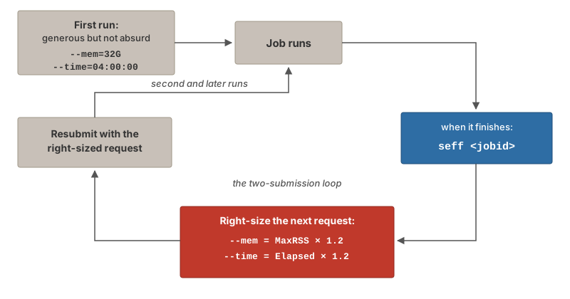
seff when the job finishes, set the next request from MaxRSS × 1.2 and Elapsed × 1.2, and resubmit.
Before treating a run as done, check two things together: seff reports State: COMPLETED with exit code 0:0, and the output file you expected exists and is complete (for example, the script’s final “Wrote …” message appears in the .out log). A job killed by OUT_OF_MEMORY or TIMEOUT mid-write leaves a truncated file on disk that looks valid but is not, and the next step in your pipeline then fails with a confusing downstream error instead of the real cause.
20.10 Interactive Jobs
For testing and development, use interactive jobs instead of batch:
The interactive partition is reserved for exactly this kind of session, with a 12-hour limit; use interactivegpu if you need a GPU to test against.
Your prompt will change from login1 to something like n049, indicating you’re on a compute node.
Interactive jobs are ideal for:
- Testing workflows before batch submission
- Debugging code
- Quick data exploration
- Running GUI applications via Open OnDemand
The discipline that goes with them: type exit the moment you are done. An interactive session holds its reserved cores and memory whether or not you are typing, and an idle session is pure waste that someone else could be using. Use an interactive session when you intend to watch the work; use sbatch for anything you intend to walk away from, because a batch job survives your laptop sleeping, your network dropping, and you logging off for the night.
20.11 Software Modules
Talapas uses the Lmod module system to manage software. This lets multiple versions coexist without conflicts.
Basic Module Commands
In Batch Scripts
Modules are loaded per shell. They do not persist between logins, and (as Section 20.7 explained) they do not travel from the login node into a batch job. Specify version numbers (R/4.3.3, not R) so that a default-version change on the cluster cannot silently change your results.
The Three Software Layers
Lmod modules are the first of three ways to get software onto Talapas, and most real projects use two of them together. Table 20.9 summarizes the trade-offs.
| Layer | What it is | Best for | Limits |
|---|---|---|---|
| Lmod modules | Centrally installed software, loaded with module load
|
Compilers, CUDA, R and Python interpreters, common tools (samtools, bwa, apptainer) |
Only what RACS has installed; versions change over time |
| Per-user environments | Packages you install into your own space: an R library (~/Rlibs) pinned with renv, or a conda/venv environment |
Your project’s R or Python packages, at exact versions | Lives in your home or project directory; must be rebuilt on another cluster |
| Containers (Apptainer) | A single image file holding an entire operating system plus software stack | Complex tool chains, exact reproduction of a published environment, moving between clusters | Larger to build; you (or a collaborator) must maintain the image |
Figure 20.7 shows how the layers combine.
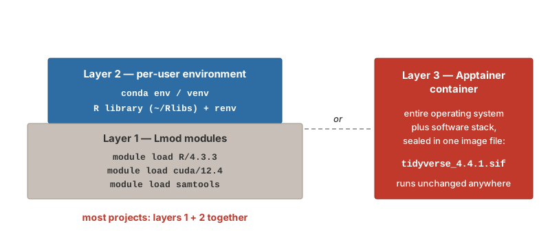
Layer 2: per-user environments. The system R and Python modules are read-only, so packages you install go into your own directory. For R, create a per-user library once and point R at it; install.packages() and BiocManager::install() will then write there:
To make a project reproducible, record the exact package versions with renv: renv::init() in the project, renv::snapshot() to write renv.lock, and renv::restore() on a fresh clone to reinstall the same versions. Commit renv.lock (not the library itself) to Git. For Python the equivalent is a conda environment (module load miniconda3/20240410, conda create -n myenv python=3.12 numpy pandas, conda activate myenv) or a venv; many bioinformatics tools are one conda install away thanks to the Bioconda channel (Grüning et al., 2018). Either way, export the environment - ideally conda env export --from-history, which records only the packages you asked for (Section 20.11.4) - and version-control the file. Activate the environment inside the job script, exactly as you load modules.
The environment.yml file is also how an environment moves to the cluster. If you recorded your project’s environment on your laptop with conda env export --from-history > environment.yml, you do not recreate it on Talapas from memory—you rebuild it from the file:
The same two lines—module load miniconda3/20240410 and conda activate—must appear inside your batch scripts, because every batch job starts with a clean shell (Section 20.7).
By default conda installs every environment, and caches every package it has ever downloaded, under your home directory—whose quota (Table 20.3) a few heavyweight environments plus the package cache can erode surprisingly quickly. Keep an eye on it: conda env list shows the environments you have accumulated, conda remove -n old_env --all deletes one you no longer need, conda clean -a clears the download cache, and df -h ~ (Section 20.5.4) tells you where you stand.
Layer 3: containers. A container packages the entire software stack, from operating-system libraries up, into one portable, versioned file. Docker (Merkel, 2014) is the standard on laptops and in the cloud, but it requires root privileges, so clusters do not run it. Apptainer (formerly Singularity) (Kurtzer et al., 2017) is its HPC-safe counterpart: it runs as an ordinary user, mounts your home and project directories automatically, and can pull Docker images directly, so an image built on a laptop runs unchanged on Talapas:
Inside a batch script the last line becomes apptainer exec /path/to/image.sif Rscript analysis.R. Containers are the strongest reproducibility guarantee available: a collaborator with the same .sif file gets the same results, on any cluster, years later.
- Just need R or Python and a few packages? Modules plus a per-user library (layers 1 + 2), pinned with
renvor anenvironment.yml. - Reproducing a published pipeline or moving between clusters? A container (layer 3), usually run with a module-provided
apptainer. - Working from a workflow manager (Section 20.14.4)? Snakemake and Nextflow can create conda environments or pull containers per step automatically.
Conda in Depth
Conda earns its place as the course default, so it is worth understanding properly. Two ideas explain almost everything about how it behaves.
An environment is a folder. Creating an environment builds a directory of software; activating it simply puts that directory first on your shell’s PATH, so its copies of python, R, or samtools answer first; deactivating removes it again. There is no magic beyond PATH manipulation—which is also why a misbehaving environment is never worth debugging: delete it (conda env remove -n NAME) and recreate it from its record file in minutes. When a tool seems to be the wrong version, the first question is always which copy answered? — which python3 or which samtools tells you.
Packages come from channels. A channel is an online repository of pre-built software. The two that matter here are conda-forge, the community channel for general scientific software, and bioconda, which distributes thousands of pre-compiled bioinformatics tools (Grüning et al., 2018)—samtools, bwa, gatk4, stacks, and far more, each one conda install away with no compiling. Configure them once, with strict priority so each package resolves from one channel consistently:
Several installers provide conda. Anaconda is the company’s ~5 GB distribution, and both it and Miniconda default to Anaconda’s commercial channel, which requires a paid license at organizations like UO. Miniforge is the lean community installer that defaults to the free conda-forge channel—it is the one to install, on your laptop and anywhere else.
The lifecycle. One environment per project, named for the project, with the Python version pinned from the start:
$ conda create -n rnaseq python=3.12 pandas matplotlib samtools   # once
$ conda activate rnaseq                                           # every session
$ conda install bcftools                 # add packages later (conda first, pip after)
$ conda list                             # what is in here, at which versions?
$ conda env list                         # all environments; * marks the active one
$ conda env remove -n rnaseq             # environments are disposable by design
Prefer conda packages over pip within an environment, and install pip stragglers last: conda packages installed after pip packages occasionally tangle dependencies, and the clean fix is always to recreate rather than repair.
A portable record. A plain conda env export lists all ~200 resolved dependencies, and such a file written on a Mac often fails to rebuild on Linux, because low-level dependencies differ by operating system. The portable form records only what you asked for, and drops the machine-specific prefix: line—this is the exact form the Talapas documentation recommends for sharing:
You can equally write one from scratch; it is just a short text file:
Keep an environment.yml in each project’s repository, next to the code: it is simultaneously your collaborator instructions, your Talapas deployment recipe, and the environment section of your methods.
Cluster particulars. Three habits specific to Talapas. If the cluster’s conda module is older and a conda create grinds for minutes, add --solver=libmamba—the fast solver that modern conda uses by default (the standalone mamba command, which you will still see in documentation, was its drop-in predecessor). RACS recommends adding a date tag to environment names on the cluster (rnaseq-20261123) so successive rebuilds of a pipeline’s environment stay distinguishable. And because environments are large and land in your quota-limited home directory by default, conda create --prefix /projects/yourPIRG/.../envs/NAME places one in project space instead, while conda clean -a reclaims the download cache anywhere.
The Environment-Tool Ecosystem
Conda is not the only environment framework, and you will meet the others constantly in tutorials, collaborators’ repositories, and cluster documentation. They fall into two families: tools that manage Python packages only, and tools that manage the full conda ecosystem of compiled software. Knowing which family a tool belongs to tells you most of what you need, and the dividing line is practical: if a workflow needs samtools or bwa, only the conda family can provide it—no amount of pip install produces a working aligner.
| Tool | What it manages | Installs from | Compiled tools? | One-line verdict |
|---|---|---|---|---|
| conda | Python/R + any compiled software | conda channels | Yes | The default for genomics and this course |
| mamba | Same (drop-in conda replacement) | conda channels | Yes | Mostly obsolete now that conda uses its solver |
| micromamba | Same, as one tiny static binary | conda channels | Yes | Conda for containers and CI pipelines |
| pixi | Conda packages, per project | conda channels + PyPI | Yes | The modern project-first take on conda |
| venv | Python packages only | PyPI (via pip) | No | Built into Python; fine for pure-Python work |
| uv | Python packages, versions, projects | PyPI | No | Very fast modern replacement for venv + pip |
| renv | R packages, per project | CRAN/Bioconductor | No | The R-world analogue; composes with conda |
A few notes beyond the table. venv (Section 12.3) ships with Python itself: an environment lives inside the project folder as .venv/, borrows your existing interpreter, and records itself in requirements.txt—when a Python tutorial says “create a virtual environment,” this is what it means. micromamba is a single self-contained binary needing no base environment or installer, which makes it the standard way to get conda packages inside Docker/Apptainer images and CI pipelines. uv is a Rust reimplementation of the whole venv-plus-pip toolchain, routinely 10–100× faster, with real project management (pyproject.toml plus a lockfile); its limit is the family line—PyPI only. pixi, from the mamba developers, installs the same packages from the same channels as conda but organizes them per project, with a pixi.toml and an exact lockfile in the repository; it is increasingly common in bioinformatics repositories, so when you meet a repo with a pixi.toml, pixi install in that directory rebuilds the authors’ exact environment. And renv (above) manages R packages per project—conda can supply a pinned R itself on a cluster, and renv pins the packages inside it, so the two compose rather than compete.
For this course and for genomics work generally: conda via Miniforge, because it is the only family that delivers bioconda’s compiled tools, it is what Talapas provides, and the environment.yml loop runs through it. File the rest as vocabulary—venv or uv when a pure-Python project calls for them, micromamba if you containerize, pixi as the likely future shape of conda-style work.
20.12 GPU Jobs
For machine learning and GPU-accelerated computing:
#!/bin/bash
#SBATCH --job-name=gpu_job
#SBATCH --partition=gpu             # GPU partition
#SBATCH --account=myPIRG
#SBATCH --time=1-00:00:00           # 1 day
#SBATCH --nodes=1
#SBATCH --gres=gpu:1                # Request 1 GPU
#SBATCH --mem=32G

# Load CUDA and your software
module load cuda/12.4
module load miniconda3/20240410

# Activate your environment
conda activate ml_env

# Run GPU code
python train_model.py
Check available GPUs:
20.13 A Complete Example
Let’s walk through a realistic bioinformatics workflow:
1. Prepare Your Script
Create genome_analysis.sh:
#!/bin/bash
#SBATCH --job-name=genome_analysis
#SBATCH --partition=compute
#SBATCH --account=myPIRG
#SBATCH --output=logs/genome_%j.out
#SBATCH --error=logs/genome_%j.err
#SBATCH --time=08:00:00
#SBATCH --cpus-per-task=8
#SBATCH --mem=32G

# Exit on error, unset variable, or failed pipeline stage
set -euo pipefail

# Load modules
module purge
module load bwa/0.7.17
module load samtools/1.17

# Set variables
GENOME="/projects/myPIRG/shared/reference/human_GRCh38.fa"
READS_R1="/projects/myPIRG/myuser/data/sample_R1.fastq.gz"
READS_R2="/projects/myPIRG/myuser/data/sample_R2.fastq.gz"
OUTPUT="/projects/myPIRG/myuser/results"

# Create output directory
mkdir -p "$OUTPUT"

# Log start time and where we landed
echo "Job $SLURM_JOB_ID starting on $(hostname) at $(date)"

# Run alignment, using the cores SLURM actually gave us
bwa mem -t "$SLURM_CPUS_PER_TASK" "$GENOME" "$READS_R1" "$READS_R2" | \
    samtools sort -@ "$SLURM_CPUS_PER_TASK" -o "$OUTPUT/aligned.bam"

# Index BAM file
samtools index "$OUTPUT/aligned.bam"

# Log completion
echo "Analysis completed at $(date)"
The alignment step uses samtools (Danecek et al., 2021; Li et al., 2009) to sort and index the BAM output; the -t and -@ thread counts come from $SLURM_CPUS_PER_TASK so that changing the #SBATCH --cpus-per-task line is the only edit needed to scale the job.
2. Submit and Monitor
# Create logs directory
$ mkdir -p logs

# Submit job
$ sbatch genome_analysis.sh
Submitted batch job 12345678

# Monitor status
$ squeue -u $USER
             JOBID PARTITION     NAME     USER  ST       TIME  NODES NODELIST(REASON)
          12345678   compute genome_a   duckid   R       5:32      1 n042

# Check output in real-time
$ tail -f logs/genome_12345678.out
Mixing Languages in One Job
A batch script is just a shell script, so nothing stops one job from running steps in different languages: load both modules, then call each interpreter in turn. This is the natural shape for a small pipeline where, say, Python summarizes raw files into a table and R turns the table into a figure:
#!/bin/bash
#SBATCH --job-name=fasta_pipeline
#SBATCH --partition=compute
#SBATCH --account=myPIRG
#SBATCH --output=logs/%x_%j.out
#SBATCH --error=logs/%x_%j.err
#SBATCH --time=01:00:00
#SBATCH --cpus-per-task=2
#SBATCH --mem=8G

set -euo pipefail

module purge
module load python3/3.11.4
module load R/4.3.3

# Step 1 (Python): summarise every FASTA file into one table
python3 fasta_stats.py data/*.fasta > results/fasta_stats.tsv

# Step 2 (R): read that table, make the figure
Rscript plot_stats.R results/fasta_stats.tsv results/fasta_stats.png
Two details carry the weight here. First, set -euo pipefail is what makes the chain safe: if the Python step fails, the job stops rather than handing R a truncated or empty table that would produce a plausible-looking but wrong figure. Second, both scripts take their file names from the command line (commandArgs(trailingOnly = TRUE) in R, sys.argv in Python) rather than hard-coding paths, so the same scripts run unchanged on your laptop and on the cluster. When the two steps grow expensive enough to need different resource requests, split them into two jobs chained with --dependency=afterok: (Table 20.4) instead.
20.14 Designing a Pipeline on the Cluster
One job is easy. Real projects are a chain of steps (align, then count, then model, then plot) run over many samples, and the cluster rewards a particular way of organizing that chain. The habits below turn a pile of scripts into a pipeline that can be re-run, resumed after a failure, and scaled from one sample to a hundred without rewriting anything. They apply whether the steps are shell, R, or Python, and they are the same habits that Chapter 21 recommends within a single R session (test sequentially first, then scale out).
Stage Data, Then Checkpoint Every Step
Stage data on fast storage. Put inputs and intermediates for a run under /scratch/<PIRG>/<duckid>/<project>/ and keep only code and final results in /projects (Section 20.5.2). Do not hard-code that location: read it from an environment variable or a small config file so the same scripts run unchanged on your laptop, on scratch, or in a collaborator’s directory.
Inside R the same idea is data_dir <- Sys.getenv("DATA_DIR", unset = "data"); in Python, os.environ.get("DATA_DIR", "data").
Write a checkpoint after every step. Each step reads a named file, does its work, and writes a new named file that the next step reads. The file is a checkpoint: a self-contained snapshot of the analysis at that stage. If step 4 fails because of a memory spike, you fix the request and rerun step 4; steps 1 through 3 are untouched. Without checkpoints, a failure anywhere forces a rerun from scratch. The cost is disk space and one discipline: verify the checkpoint (State: COMPLETED, output present and complete) before launching the step that consumes it.
Skip work that is already done. Once outputs are checkpoints, the script can test for them and move on, which makes re-running the whole pipeline after a partial failure safe and cheap:
if [[ -s "$DATA_DIR/aligned/${SAMPLE}.bam" ]]; then
    echo "$SAMPLE already aligned, skipping"
else
    bwa mem -t "$SLURM_CPUS_PER_TASK" "$GENOME" "$R1" "$R2" \
        | samtools sort -@ "$SLURM_CPUS_PER_TASK" -o "$DATA_DIR/aligned/${SAMPLE}.bam.tmp"
    mv "$DATA_DIR/aligned/${SAMPLE}.bam.tmp" "$DATA_DIR/aligned/${SAMPLE}.bam"
fi
Writing to a .tmp name and renaming only after success means a job killed mid-write never leaves a truncated file that the -s test would mistake for a finished one.
Log Everything, Test on a Subset, Then Scale Out
Log everything. A batch job has no terminal, so its logs are your only window into what happened. Print a line at the start (echo "Job $SLURM_JOB_ID on $(hostname), $(date)"), one per major step, and one at the end (“Wrote …”), and keep --output/--error in a logs/ directory named with %x_%j so you can match a log to a job weeks later. Record software versions too (module list 2>&1, R --version, samtools --version), because “which version did I use?” is the first question a reviewer asks.
Test on a subset first. Before submitting a 12-hour job, run the script on a tiny input: the first 100,000 reads (zcat R1.fastq.gz | head -n 400000 | gzip > test_R1.fastq.gz), one chromosome, one sample. Run it in an interactive session (Section 20.10) where you can watch it fail quickly. Only when the small run finishes cleanly and seff gives you a resource profile should you submit the full-size job with right-sized requests (Section 20.9).
Scale out with job arrays, not copies of the script. When the same step must run on many samples, do not write one script per sample. Write one script and submit it as a job array.
Job Arrays: One Script, Many Samples
--array=1-N submits N independent sub-jobs from a single script, each with its own $SLURM_ARRAY_TASK_ID (1 through N) and its own log, time limit, and resource accounting. The script uses the task ID to pick a sample from a list, so adding a sample means adding a line to samples.txt, not editing code:
#!/bin/bash
#SBATCH --job-name=align
#SBATCH --partition=compute
#SBATCH --account=myPIRG
#SBATCH --time=02:00:00
#SBATCH --cpus-per-task=8
#SBATCH --mem=16G
#SBATCH --array=1-24%8               # 24 samples, at most 8 running at once
#SBATCH --output=logs/%x_%A_%a.out   # %A = array job ID, %a = task ID
#SBATCH --error=logs/%x_%A_%a.err

set -euo pipefail
module purge
module load bwa/0.7.17 samtools/1.17

# Line N of samples.txt is this task's sample
SAMPLE=$(sed -n "${SLURM_ARRAY_TASK_ID}p" samples.txt)
echo "Task $SLURM_ARRAY_TASK_ID: aligning $SAMPLE on $(hostname)"

R1="$DATA_DIR/raw/${SAMPLE}_R1.fastq.gz"
R2="$DATA_DIR/raw/${SAMPLE}_R2.fastq.gz"
OUT="$DATA_DIR/aligned/${SAMPLE}.bam"

if [[ -s "$OUT" ]]; then
    echo "$SAMPLE already done"; exit 0
fi
bwa mem -t "$SLURM_CPUS_PER_TASK" "$GENOME" "$R1" "$R2" \
    | samtools sort -@ "$SLURM_CPUS_PER_TASK" -o "$OUT.tmp"
mv "$OUT.tmp" "$OUT"
samtools index "$OUT"
echo "Wrote $OUT"
Submit it with sbatch --export=ALL,DATA_DIR=/scratch/myPIRG/$USER/proj,GENOME=/projects/myPIRG/shared/ref.fa align.sh, or set those variables in the script. The %8 throttle limits how many tasks run at once, which keeps you under per-user QOS caps (Table 20.7) and leaves room for other users. Each task is right-sized independently, so a failure in sample 17 does not touch the other 23, and resubmitting the array skips the samples whose BAM already exists. Chain steps with --dependency=afterok:<array job ID> so the counting step starts only when every alignment task has succeeded.
Workflow Managers: Snakemake and Nextflow
Shell scripts with checkpoints and arrays are a hand-rolled version of what a workflow manager automates. Both Snakemake (Mölder et al., 2021) and Nextflow (Di Tommaso et al., 2017) describe a pipeline as a graph of steps connected by their input and output files. The manager works out the order, re-runs only steps whose inputs changed or whose outputs are missing, runs independent branches in parallel, and, crucially for this chapter, submits each step to SLURM for you with per-step resource requests. Both can also create a conda environment (Grüning et al., 2018) or pull a container (Kurtzer et al., 2017) for each step, which takes care of the software layers in Section 20.11.3.
Snakemake uses a Python-flavored Snakefile of rules. Each rule names its inputs, outputs, and the command that turns one into the other; wildcards ({sample}) let one rule cover every sample:
SAMPLES = [line.strip() for line in open("samples.txt")]

rule all:
    input: expand("aligned/{sample}.bam.bai", sample=SAMPLES)

rule align:
    input:
        r1 = "raw/{sample}_R1.fastq.gz",
        r2 = "raw/{sample}_R2.fastq.gz",
        ref = "ref/genome.fa"
    output: "aligned/{sample}.bam"
    threads: 8
    resources: mem_mb = 16000, runtime = 120
    shell:
        "bwa mem -t {threads} {input.ref} {input.r1} {input.r2} "
        "| samtools sort -@ {threads} -o {output}"

rule index:
    input: "aligned/{sample}.bam"
    output: "aligned/{sample}.bam.bai"
    shell: "samtools index {input}"
Run it on Talapas with the SLURM executor plugin: snakemake --executor slurm --jobs 20 --default-resources slurm_account=myPIRG slurm_partition=compute. Snakemake submits one job per rule instance, waits for them, and stops if anything fails; rerunning the same command afterwards picks up where it left off.
Nextflow uses processes connected by channels (streams of files). The same pipeline looks like this:
process ALIGN {
    cpus 8
    memory '16 GB'
    time '2h'

    input:
    tuple val(sample), path(r1), path(r2)
    path ref

    output:
    tuple val(sample), path("${sample}.bam")

    script:
    """
    bwa mem -t ${task.cpus} ${ref} ${r1} ${r2} \\
        | samtools sort -@ ${task.cpus} -o ${sample}.bam
    """
}

workflow {
    reads = Channel.fromFilePairs("raw/*_R{1,2}.fastq.gz")
                   .map { id, files -> tuple(id, files[0], files[1]) }
    ALIGN(reads, file("ref/genome.fa"))
}
A short nextflow.config with process.executor = 'slurm' and process.clusterOptions = '--account=myPIRG --partition=compute' sends every process to SLURM; nextflow run main.nf -resume reuses cached results after a failure. Nextflow’s main attraction is the nf-core collection of community-maintained, tested pipelines (RNA-seq, variant calling, ATAC-seq, and dozens more) that you can run on Talapas with a single command and a sample sheet.
For a handful of steps on one dataset, a well-written shell script with checkpoints is clear and sufficient. Once a pipeline grows past that, or must run on many datasets, the learning investment in a workflow manager pays for itself in the first rerun.
20.15 Sharing Files with Your Lab Group
On your laptop you are usually the only user, so the permission system (Section 6.2) mostly matters for making scripts executable. On Talapas it becomes the tool you share with: every file belongs to a group, and the group’s permissions decide which of your labmates can read or edit your work.
Your Talapas account belongs to one or more PIRGs (Principal Investigator Research Groups), and each PIRG has shared space under /projects/:
Three commands cover almost all day-to-day sharing:
The capital X is a small but important refinement of what you learned in Section 6.2.2: it adds execute permission only to directories (and to files that are already executable), so a recursive chmod does not accidentally mark every data file as a program.
The same system protects data from your collaborators as well as sharing it with them:
Two conventions make all this painless. First, your home directory on Talapas is private by default—work meant for the lab belongs in your PIRG’s /projects/ space, not in $HOME. Second, agree with your lab on group-writable directories before a deadline, not during one; if files created in shared space keep arriving with the wrong group, ask RACS about setting the directory’s setgid bit so new files inherit the project group automatically.
20.16 Best Practices
Do
- Request only the resources you need, and check
seffafter every job - Test with small datasets first, in an interactive session
- Use
--timeconservatively (but not too short) - Start every job script with
set -euo pipefailand load modules inside it - Put large intermediates in
/scratchand results you care about in/projects - Clean up old files regularly, and keep your own backups
- Document your workflows and record software versions
- Acknowledge RACS in publications
Don’t
- Run heavy computation on login nodes
- Leave idle interactive sessions or Open OnDemand apps running
- Store sensitive data without encryption
- Ignore error messages
- Request maximum resources or the
memorypartition “just in case” - Leave anything you would miss in
/scratch
Acknowledgment
When publishing research using Talapas, include this acknowledgment:
“The authors acknowledge Research Advanced Computing Services (RACS) at the University of Oregon for providing computing resources that have contributed to the research results reported within this publication.”
20.17 Getting Help
Resources
- Documentation: uoracs.github.io/talapas2-knowledge-base
- Service Desk: hpcrcf.atlassian.net/servicedesk
- Email: racs@uoregon.edu
- Office Hours: Knight Library, Dream Lab 122E (Wednesdays 1-3pm)
20.18 Running Example: The Stickleback Data
This section applies the chapter to the course dataset described in Section 1.5 (80 stickleback, 4 treatment groups, 600 genes). The same steps appear on the Week 10 slides, so the book and the lecture can be read side by side.
Nothing about an analysis has to change to run on Talapas; what changes is where it runs and who starts it. Put the pipeline from Chapter 14 in a script, stickle_means.R, that reads the data file and writes results/gene_means.tsv. Then wrap it in a SLURM batch script that asks for modest resources, loads R, and runs it:
#!/bin/bash
#SBATCH --job-name=stickle_means
#SBATCH --account=<your_pirg>
#SBATCH --partition=compute
#SBATCH --time=00:10:00
#SBATCH --mem=4G
#SBATCH --cpus-per-task=1
#SBATCH --output=logs/stickle_%j.out
#SBATCH --error=logs/stickle_%j.err

module load R/4.4.0
cd ~/projects/comptools
Rscript stickle_means.R data/Stickle_RNAseq.tsv results/gene_means.tsv
Submit it, watch it in the queue, and read what it wrote:
A 160 KB file does not need a cluster, of course, and the job will finish in seconds. The point is the pattern: the same Rscript call you ran on your laptop, launched by sbatch instead of by you, with its output in a log file you read afterwards. For the term project, the identical pattern handles files a thousand times larger, and Chapter 21 shows how to use more than one core when it does.
20.19 Summary
High-performance computing extends your analytical capabilities beyond personal computers:
- Talapas provides 14,520+ CPU cores, 89 GPUs, 129 TB of memory, and about 3 PB of storage
- Connect via SSH (with or without the VPN), Remote-SSH from VS Code or Positron, or the Open OnDemand web interface
- SLURM manages job scheduling and resource allocation; fair-share and backfill mean honestly sized jobs start sooner
- Batch scripts combine
#SBATCHresource requests with your commands; useset -euo pipefail, load modules inside the script, and read$SLURM_*variables instead of hard-coding -
seffandsaccttell you what a job actually used; right-size the next run fromMaxRSSandElapsed - Software comes in three layers: Lmod modules, per-user environments (
renv, conda), and Apptainer containers -
/scratchis fast but purged after 90 days; nothing on Talapas is backed up - Pipelines on the cluster stage data, checkpoint every step, log everything, test on a subset, and scale out with job arrays or a workflow manager
- Responsible use ensures fair access for everyone
Start simple—submit small test jobs, verify they work, then scale up. The HPC learning curve is real, but the capability it provides is essential for modern computational research.
For a complete reference of SLURM commands and batch script directives, see Appendix I.
Additional Reading
For more on HPC and cluster computing:
- Talapas Knowledge Base — Official UO documentation for Talapas
- SLURM Documentation — The official SLURM workload manager documentation
- HPC Carpentry — Introductory HPC lessons for researchers
- Introduction to High-Performance Scientific Computing — Comprehensive textbook on HPC concepts
For workflow management and reproducible environments at scale:
- Snakemake for HPC (Mölder et al., 2021) — Running Snakemake workflows on clusters
- Nextflow Executors (Di Tommaso et al., 2017) — Running Nextflow on SLURM and other schedulers; nf-core for ready-made pipelines
- Apptainer documentation (Kurtzer et al., 2017) — Containers on HPC, including how to pull Docker images (Merkel, 2014)
- Bioconda (Grüning et al., 2018) — Conda channel with thousands of bioinformatics tools
- The scheduler’s original design is described by Yoo, Jette, and Grondona (Yoo et al., 2003)
Exercises
Exercise 1: First Connection
- Log into Talapas via SSH
- Check which login node you’re on with
hostname - Explore your home directory and check your quota
- Find your project directory
Exercise 2: Module Practice
- Search for available R versions
- Load R and verify with
R --version - Search for Python versions
- Create a script that loads both R and Python
Exercise 3: Interactive Job
- Start an interactive session with 2 CPUs and 4GB memory
- Note how your prompt changes
- Run a simple R command
- Exit the interactive session
Exercise 4: Batch Job
- Write a batch script that:
- Requests 1 hour, 2 CPUs, 8GB memory
- Starts with
set -euo pipefailand loads R inside the script - Runs a simple R script that generates a plot
- Submit the job
- Monitor its progress
- Examine the output files, then run
seffon the job. What was the memory efficiency? What would you request next time?
Exercise 5: Job Array
- Create
samples.txtwith five made-up sample names - Write an array job (
--array=1-5) that reads its sample name withsed -n "${SLURM_ARRAY_TASK_ID}p" samples.txtand writesresults/<sample>.txtcontaining the hostname and date - Use
%A_%ain the log names and confirm you get five separate logs - Delete two of the result files and resubmit. Add a skip-if-exists test so only those two are recomputed