Lecture 06
R and Python Fundamentals 2: Data Frames, the Tidyverse and Figures
2026-11-02
Example 1 - a panel of figures
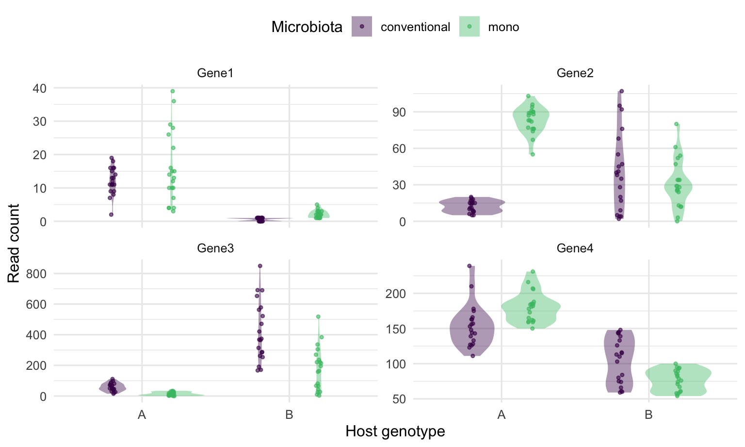
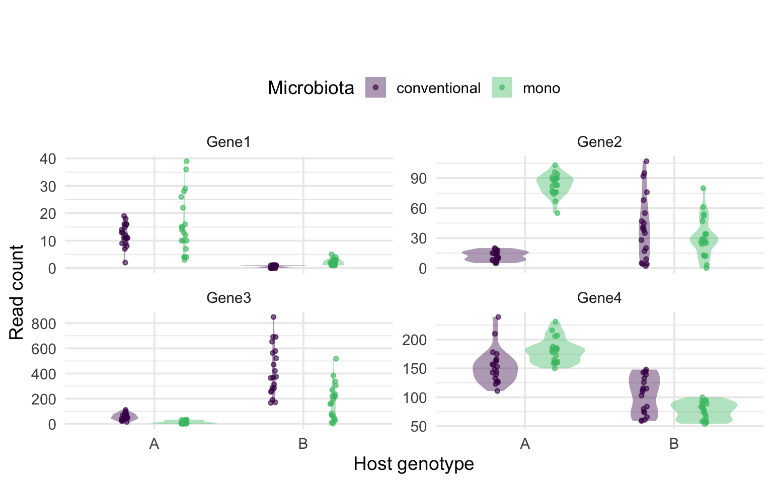
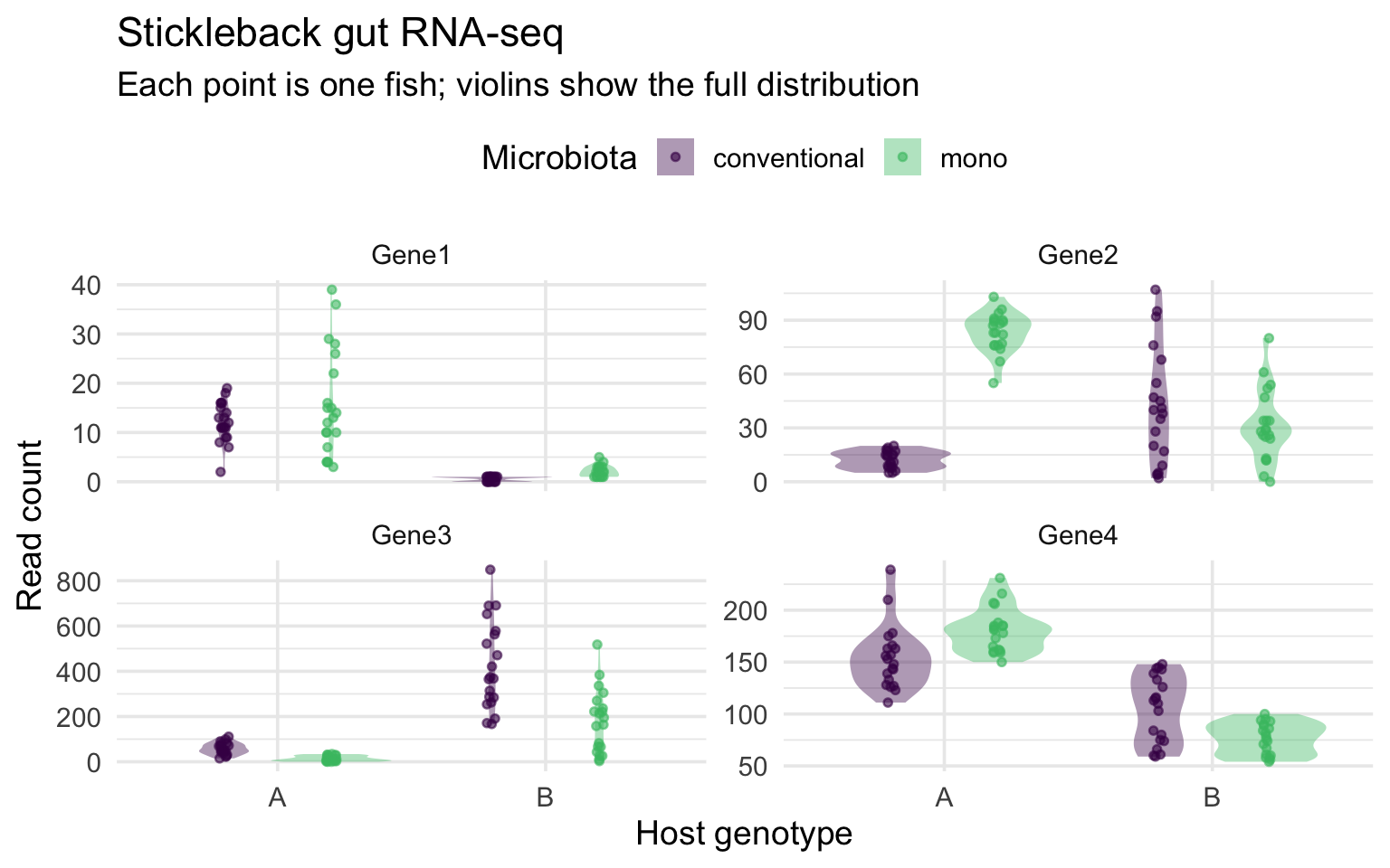
Figure 1: Read Counts of Four Genes. RNA-seq read counts for Gene1-Gene4 in n = 80 threespine stickleback (20 fish per host genotype x microbiota combination), split by host genotype and colored by microbiota treatment. Violins show each group’s full count distribution; each point is one fish, jitter-dodged to reduce overplotting. Panel y-axes are scaled independently.
Example 2 - A range of 600 genes at once
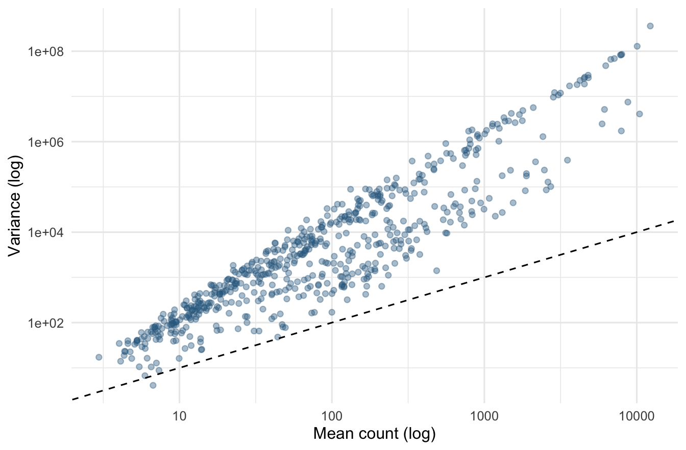
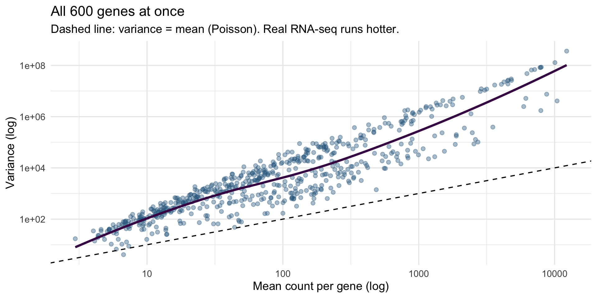
Figure 2: The mean-variance relationship for all 600 genes. Each point is one gene, placed by the mean and the variance of its read counts across the 80 fish, on log-log axes. The dashed line marks variance = mean, the expectation under Poisson sampling; nearly all genes fall above it, the overdispersion typical of RNA-seq counts.
Three distributions, drawn and plotted
set.seed(2026); n <- 2000
dir.create("results", showWarnings = FALSE)                 # the folder must exist
svg("results/distributions.svg", width = 10, height = 3.6)   # open the file device
par(mfrow = c(1, 3), mar = c(4, 4, 2, 1))      # a 1 x 3 grid of panels
hist(runif(n, 0, 100),  breaks = 40, col = "#31688e", border = "white",
     main = "Uniform(0, 100)",  xlab = "value")
hist(rnorm(n, 50, 10),  breaks = 40, col = "#440154", border = "white",
     main = "Normal(50, 10)",   xlab = "value")
hist(rpois(n, 5),       breaks = seq(-0.5, 20.5, 1), col = "#35b779",
     border = "white", main = "Poisson(5)",    xlab = "count")
dev.off()                                       # close it - the file is written
import numpy as np
import matplotlib.pyplot as plt
from pathlib import Path
rng = np.random.default_rng(2026)
n = 2000
Path("results").mkdir(exist_ok=True) # the folder must exist
draws = {"Uniform(0, 100)": (rng.uniform(0, 100, n), "#31688e"),
"Normal(50, 10)": (rng.normal(50, 10, n), "#440154"),
"Poisson(5)": (rng.poisson(5, n), "#35b779")}
fig, ax = plt.subplots(1, 3, figsize=(10, 3.6)) # the grid, as an array of axes
for a, (name, (d, c)) in zip(ax, draws.items()):
a.hist(d, bins=40, color=c, edgecolor="white")
a.set_title(name)
fig.tight_layout()
plt.savefig("results/distributions.svg")
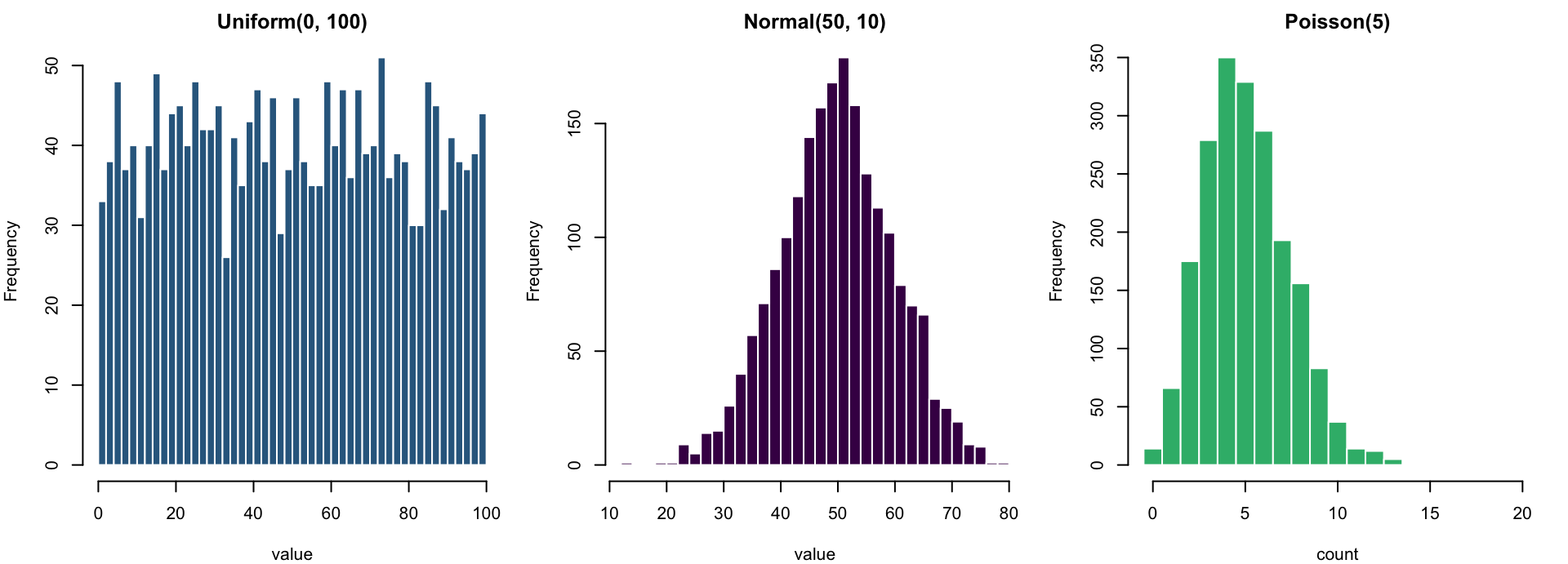
plt.show()- Same machine, three settings: uniform spreads flat, normal mounds around its mean, Poisson is discrete counts piling near
lambda - Base R saves differently from ggplot: open a file device → plot →
dev.off()- forgetdev.off()and the file is empty par(mfrow = c(1, 3))splits the plotting device into panels; eachhist()call fills the next one (plt.subplots(1, 3)hands Python the grid as an array of axes)- Change
n, the parameters andbreaks- this one figure is a little simulation lab (notebook sections 8-10)
The tidyverse family of packages
- A family of R packages that share one grammar: data frames in, data frames out
- Loading
tidyverseloads all of them at once
The grammar of graphics: a plot is a stack of layers
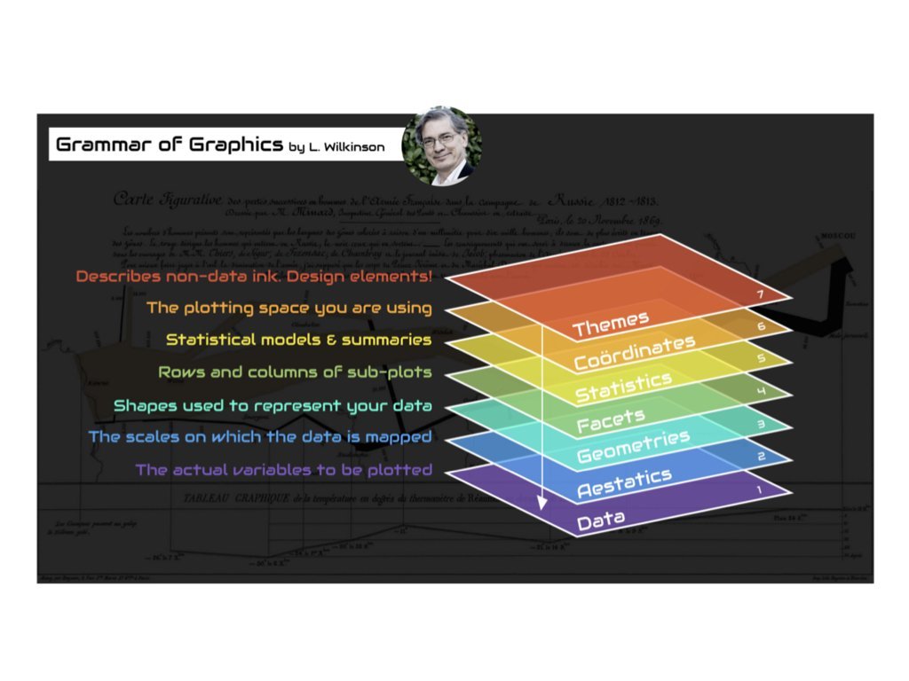
Building a figure layer by layer: 1 - data, aesthetics, a geom
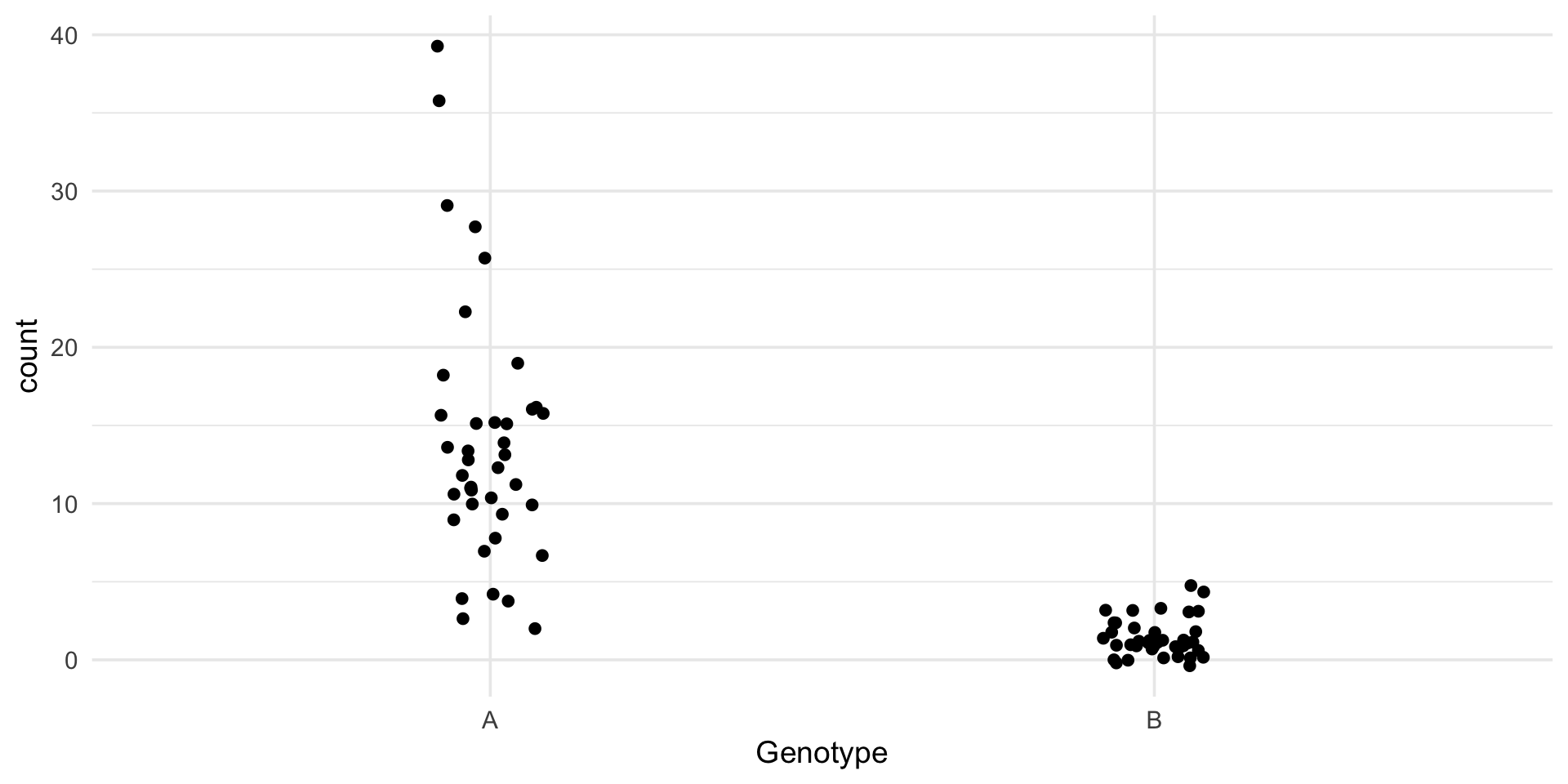
ggplot(data, aes(...))declares the mapping: which column drives which visual channel- A geom draws it;
geom_jitter()isgeom_point()plus sideways noise - Nothing is styled yet - and it is already a readable figure
- The save-line convention: every example in this deck ends by writing the figure to
results/as an SVG -ggsave()for ggplot,plt.savefig()in Python
Building a figure layer by layer: 2 - more aesthetics, more geoms
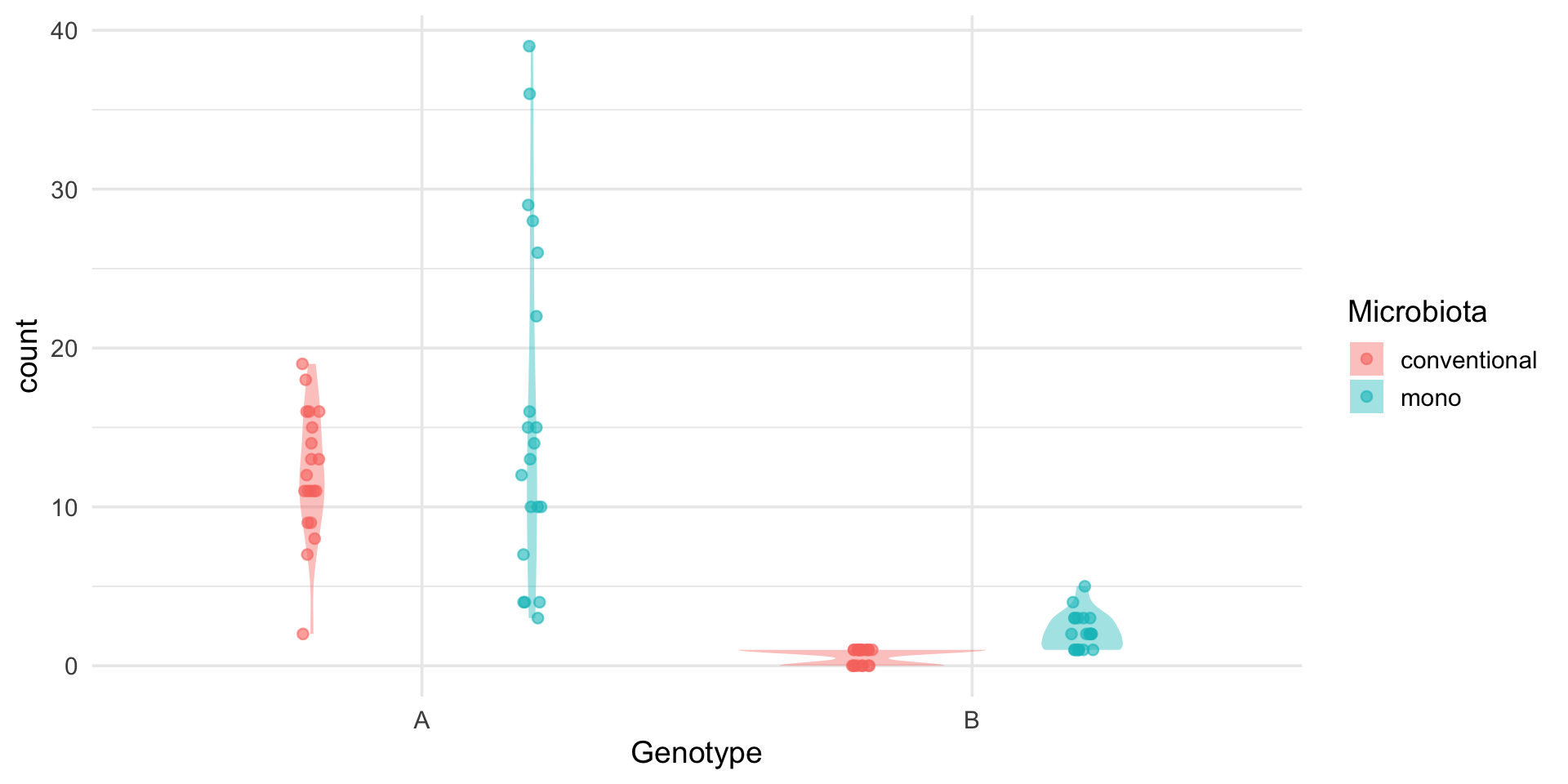
ggplot(gene1, aes(x = Genotype, y = count, fill = Microbiota)) +
  geom_violin(alpha = 0.4, color = NA, position = position_dodge(0.8)) +
  geom_point(aes(color = Microbiota), alpha = 0.6,
             position = position_jitterdodge(jitter.width = 0.08, dodge.width = 0.8))

ggsave("results/gene1_violin.svg", width = 7, height = 5)- Mapping a column to
fill/color(huein seaborn) splits the groups and builds the legend - automatically, from the data - Layers draw in order: violin first, points on top
position_dodgeplaces the two microbiota groups side by side
Building a figure layer by layer: 3 - facets, scales, labels, theme
stickle_long |>
  filter(gene %in% paste0("Gene", 1:4)) |>
  ggplot(aes(Genotype, count, fill = Microbiota)) +
  geom_violin(alpha = 0.4, color = NA, position = position_dodge(0.8)) +
  geom_point(aes(color = Microbiota), alpha = 0.6, size = 1.2,
             position = position_jitterdodge(jitter.width = 0.08, dodge.width = 0.8)) +
  scale_fill_viridis_d(end = 0.7) + scale_color_viridis_d(end = 0.7) +
  facet_wrap(~ gene, scales = "free_y") +
  labs(x = "Host genotype", y = "Read count",
       title = "Stickleback gut RNA-seq",
       subtitle = "Each point is one fish; violins show the full distribution") +
  theme_minimal(base_size = 14) + theme(legend.position = "top")

ggsave("results/gene_panel.svg", width = 8, height = 5)
long4 = stickle_long[stickle_long["gene"].isin([f"Gene{i}" for i in range(1, 5)])]
g = sns.catplot(data=long4, x="Genotype", y="count", hue="Microbiota",
col="gene", col_wrap=2, kind="violin", inner="point",
palette=["#440154", "#35b779"], sharey=False, height=2.6, aspect=1.3)
g.set_axis_labels("Host genotype", "Read count")
g.set_titles("{col_name}")
g.figure.suptitle("Stickleback gut RNA-seq", y=1.02)
plt.savefig("results/gene_panel.svg", bbox_inches="tight")
plt.show()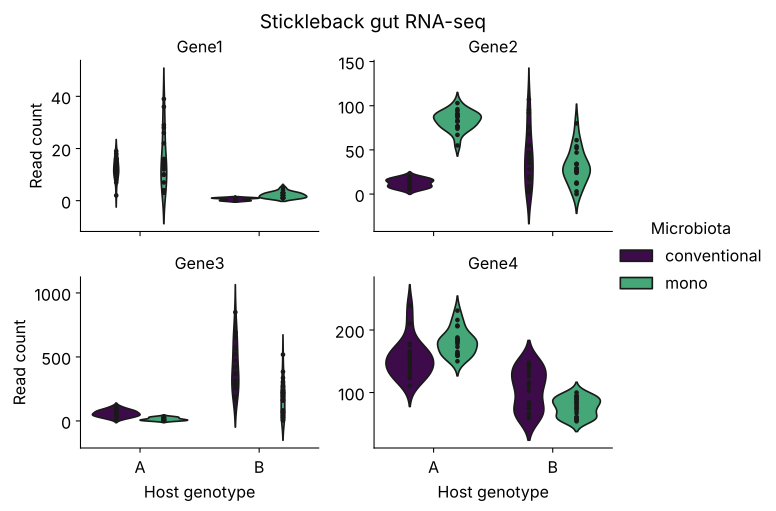
facet_wrap(~ gene)- one panel per gene, for free;scales = "free_y"lets each gene keep its own axis- This is Figure 1 from the start of class - and the last line of the code writes it to
results/gene_panel.svg
Geom example 1: geom_histogram()
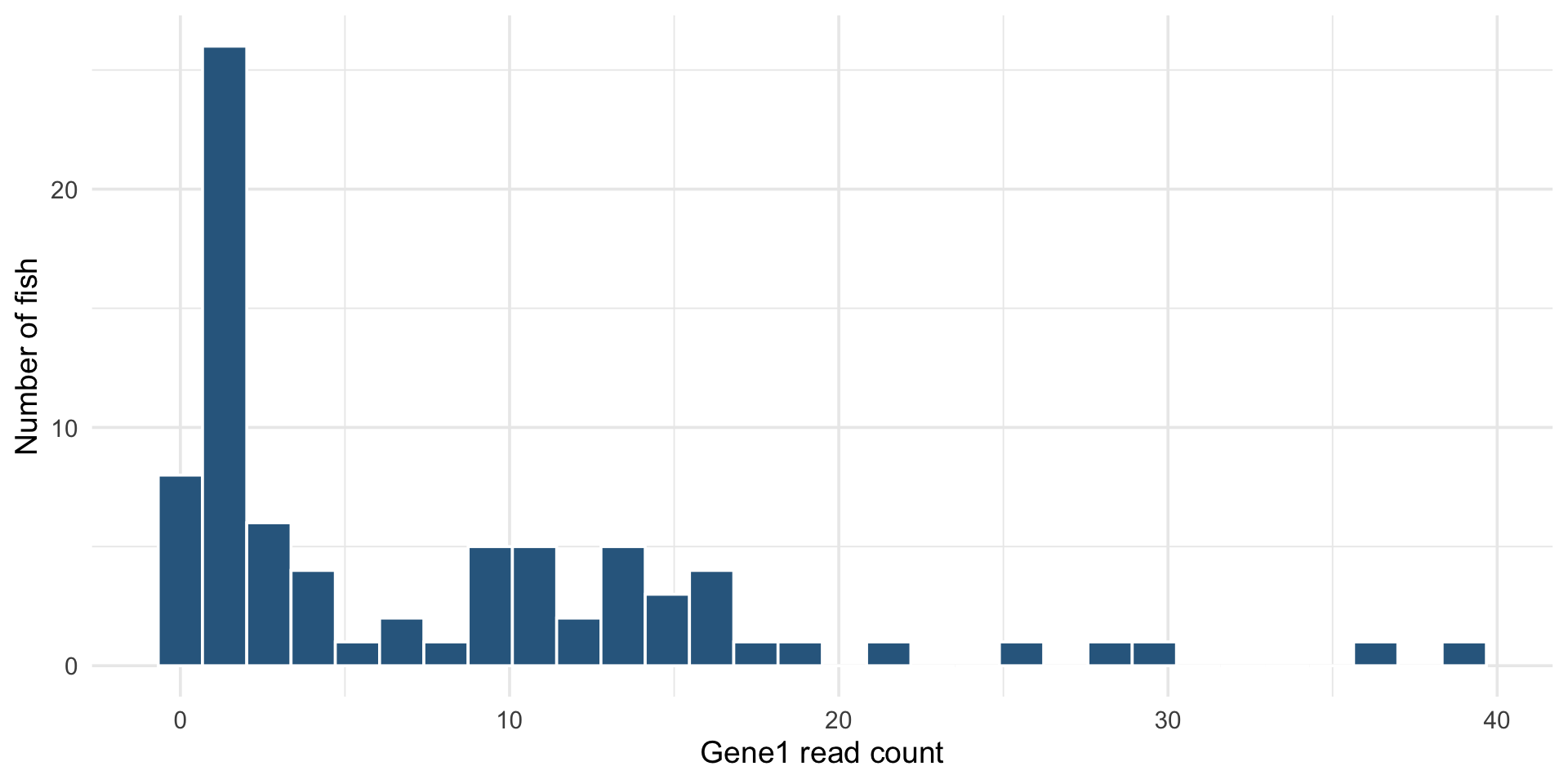
- One continuous column mapped to
x; the geom does the binning binschanges the story - always try a few values- The smooth cousin is
geom_density()
Geom example 2: geom_boxplot()
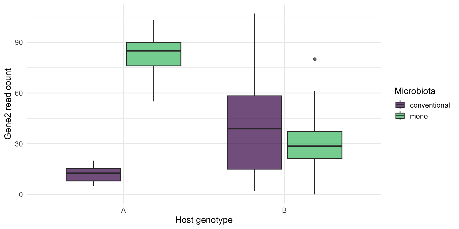
- Continuous by category: the five-number summary per group, at a glance
- A second categorical variable maps to
fill/hueand dodges automatically - When the shape of the distribution matters, swap in
geom_violin()(as in Figure 1)
Geom example 3: geom_point()
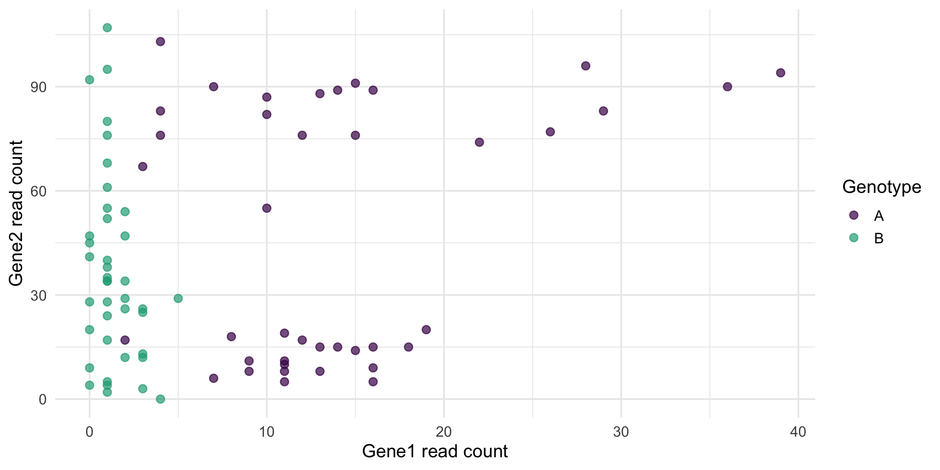
- Two continuous columns: the workhorse for relationships between variables
- A third column rides along as
color- no extra work - With thousands of points, lower
alphaso density shows through
Geom example 4: geom_smooth()
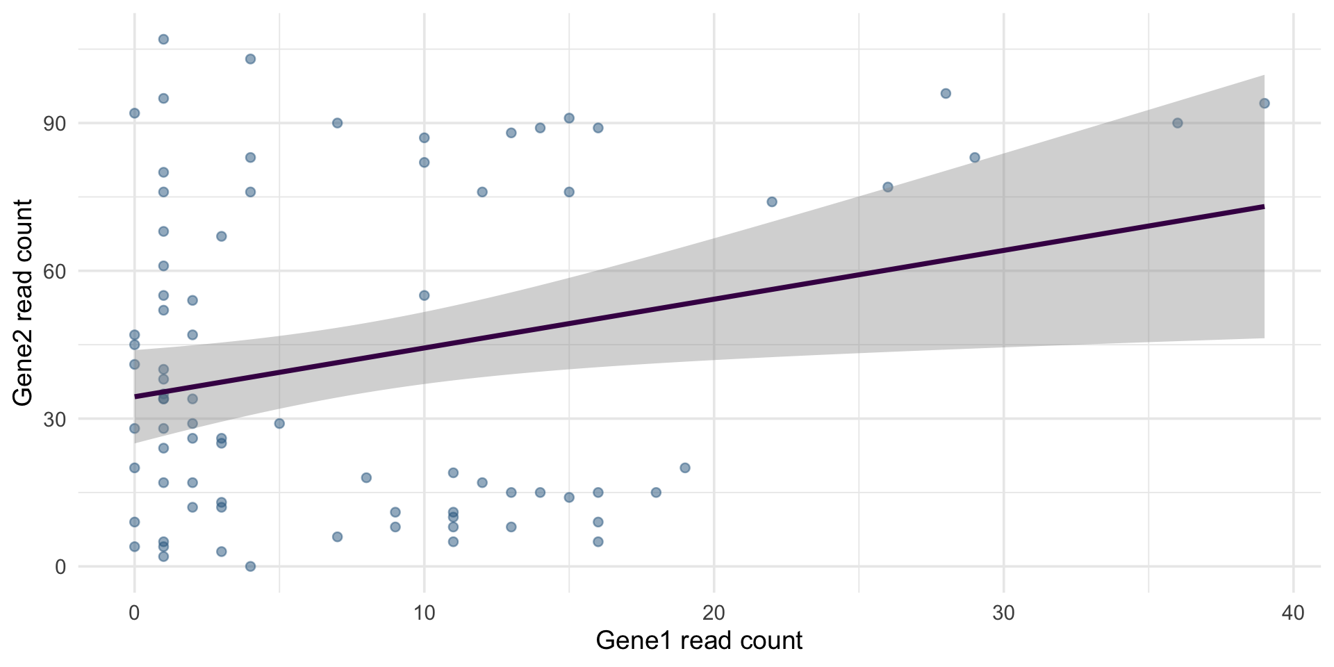
- A trend is just another layer on the scatter - that is the grammar at work
method = "lm"fits a straight line (with its confidence ribbon); the default is a flexible loess curve- The fitted line previews the statistics sequence: this is a regression
Geom example 5: geom_line()
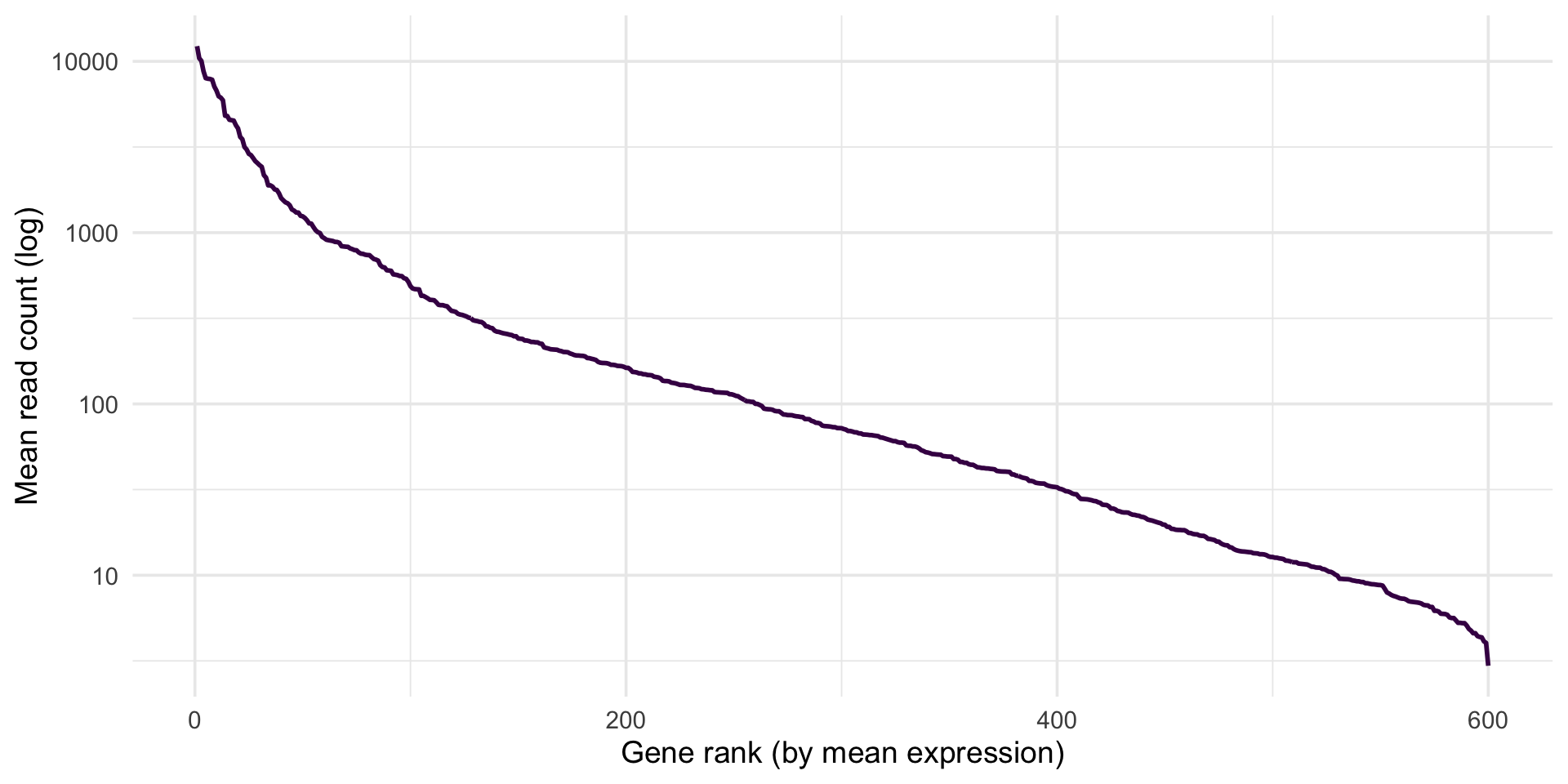
stickle_long |>
group_by(gene) |>
summarize(mean_count = mean(count)) |>
arrange(desc(mean_count)) |>
mutate(rank = row_number()) |>
ggplot(aes(x = rank, y = mean_count)) +
geom_line(color = "#440154", linewidth = 1) +
scale_y_log10() +
labs(x = "Gene rank (by mean expression)", y = "Mean read count (log)")
ggsave("results/gene_rank_means.svg", width = 7, height = 5)genes = [c for c in stickle.columns if c.startswith("Gene")]
means = stickle[genes].mean().sort_values(ascending=False)
fig, ax = plt.subplots()
ax.plot(range(1, len(means) + 1), means, color="#440154", lw=2)
ax.set(yscale="log", xlabel="Gene rank (by mean expression)",
ylabel="Mean read count (log)")
plt.savefig("results/gene_rank_means.svg")
plt.show()- Lines need an ordered x - time, position, or (here) rank; connecting unordered categories draws meaningless slopes
- The shape is classic transcriptomics: a few genes dominate, then a long tail - which is why the log scale is essential
- The whole pipeline is dplyr verbs feeding the plot:
group_by |> summarize |> arrange |> mutate |> ggplot
Geom example 6: geom_col()
gene1 |>
group_by(Genotype, Microbiota) |>
summarize(median_count = median(count), .groups = "drop") |>
ggplot(aes(x = Genotype, y = median_count, fill = Microbiota)) +
geom_col(position = "dodge") +
scale_fill_viridis_d(end = 0.7) +
labs(x = "Host genotype", y = "Median Gene1 read count")
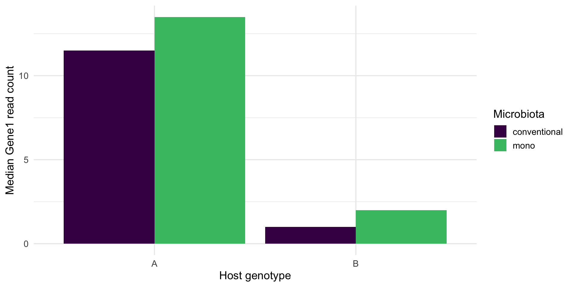
ggsave("results/gene1_group_medians.svg", width = 7, height = 5)geom_bar()counts rows for you;geom_col()plots values you computed - here, the group medians fromsummarize()- Bars start at zero by construction, which keeps magnitudes honest
- A bar hides the distribution behind one number - prefer boxplots or violins when the spread matters
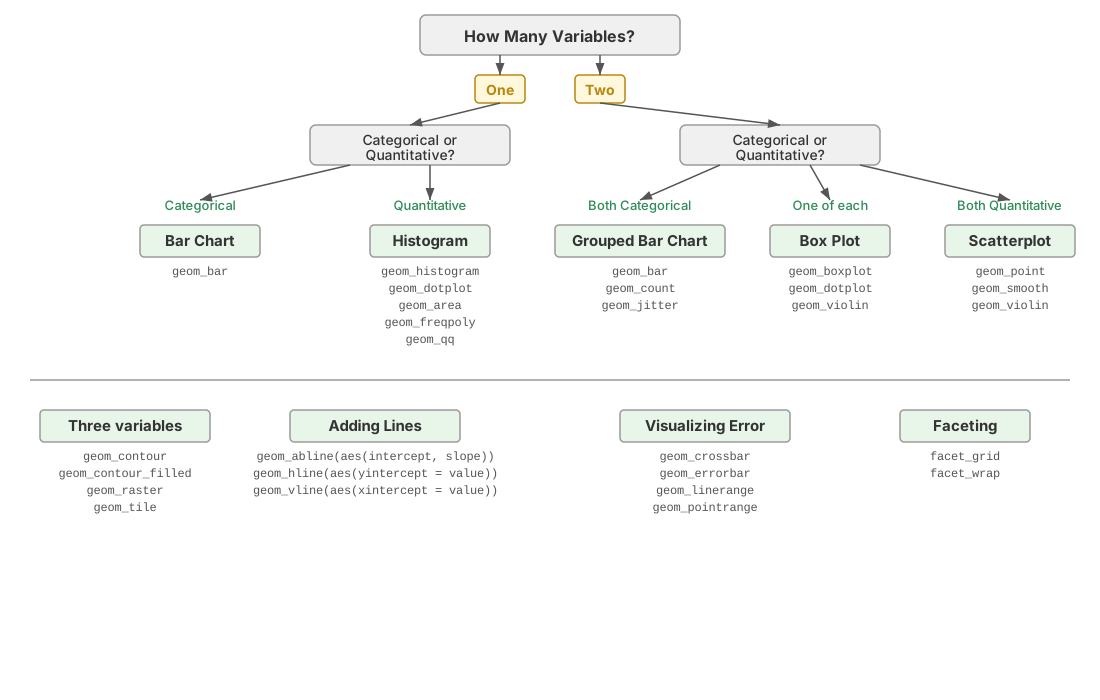
Choosing the right kind of plot
Four genes in one figure
library(tidyverse)
stickle <- read_tsv("data/Stickle_RNAseq.tsv", show_col_types = FALSE) |>
rename(geno_micro = `Geno&Micro`)
stickle_long <- stickle |>
pivot_longer(starts_with("Gene"), names_to = "gene", values_to = "count")
stickle_long |>
filter(gene %in% paste0("Gene", 1:4)) |>
ggplot(aes(Genotype, count, fill = Microbiota)) +
geom_violin(alpha = 0.4, color = NA, position = position_dodge(0.8)) +
geom_point(aes(color = Microbiota), alpha = 0.6, size = 1.2,
position = position_jitterdodge(jitter.width = 0.08, dodge.width = 0.8)) +
scale_fill_viridis_d(end = 0.7) + scale_color_viridis_d(end = 0.7) +
facet_wrap(~ gene, scales = "free_y") +
labs(x = "Host genotype", y = "Read count",
title = "Stickleback gut RNA-seq",
subtitle = "Each point is one fish; violins show the full distribution") +
theme_minimal(base_size = 14) + theme(legend.position = "top")
ggsave("results/gene_panel.svg", width = 8, height = 6)import pandas as pd
import seaborn as sns
import matplotlib.pyplot as plt
stickle = pd.read_csv("data/Stickle_RNAseq.tsv", sep="\t")
stickle_long = stickle.melt(
id_vars=["Individual", "Genotype", "Microbiota", "Geno&Micro"],
var_name="gene", value_name="count")
long4 = stickle_long[stickle_long["gene"].isin([f"Gene{i}" for i in range(1, 5)])]

g = sns.catplot(data=long4, x="Genotype", y="count", hue="Microbiota",
                col="gene", col_wrap=2, kind="violin", inner="point",
                palette=["#440154", "#35b779"], sharey=False, height=2.6, aspect=1.3)
g.set_axis_labels("Host genotype", "Read count")
g.set_titles("{col_name}")
g.figure.suptitle("Stickleback gut RNA-seq", y=1.02)
plt.savefig("results/gene_panel.svg", bbox_inches="tight")
plt.show()
- This is Example 1 from the start of class, now as one complete, visible script: read the raw TSV →
renamethe awkward column →pivot_longer→ filter → plot → save - Every line was derived earlier today: the reshape in the tidyverse section, each plot layer in the build-up slides
- About 20 lines, exactly as promised - and swapping the four gene names reuses it for any genes (Ex 6 asks you to do exactly that)
All 600 genes in one figure
stickle_long |>
  group_by(gene) |>
  summarize(mean = mean(count), var = var(count)) |>
  ggplot(aes(mean, var)) +
  geom_point(alpha = 0.4, color = "#31688e") +
  geom_abline(slope = 1, intercept = 0, linetype = "dashed") +
  geom_smooth(se = FALSE, color = "#440154") +
  scale_x_log10() + scale_y_log10() +
  labs(x = "Mean count per gene (log)", y = "Variance (log)",
       title = "All 600 genes at once",
       subtitle = "Dashed line: variance = mean (Poisson). Real RNA-seq runs hotter.") +
  theme_minimal(base_size = 14)

ggsave("results/mean_variance.svg", width = 7, height = 5)
import numpy as np
genes = [c for c in stickle.columns if c.startswith("Gene")]
mv = pd.DataFrame({"mean": stickle[genes].mean(), "var": stickle[genes].var()})
fig, ax = plt.subplots()
ax.scatter(mv["mean"], mv["var"], s=10, alpha=0.4, color="#31688e")
lims = np.array([mv["mean"].min() / 2, mv["mean"].max() * 2])
ax.plot(lims, lims, ls="--", color="black") # variance = mean
ax.set(xscale="log", yscale="log",
xlabel="Mean count per gene (log)", ylabel="Variance (log)",
title="All 600 genes at once")
plt.savefig("results/mean_variance.svg")
plt.show()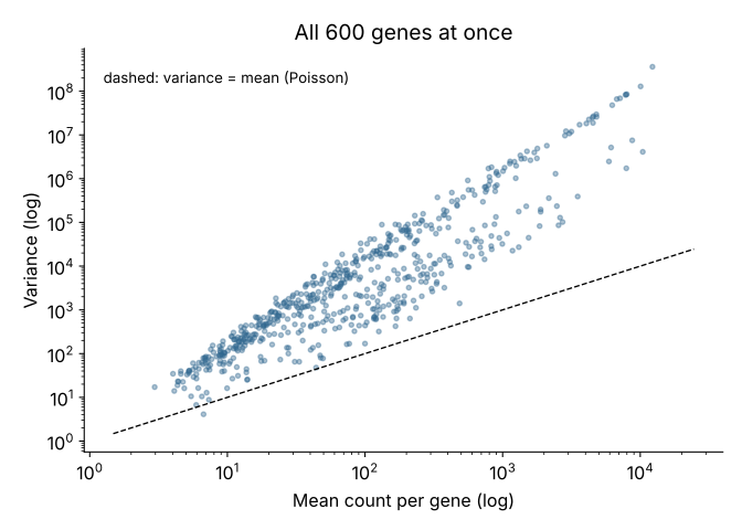
group_by(gene) |> summarize()collapses 48,000 rows to 600 - one point per gene- The biology in one glance: variance outruns the mean, which is why RNA-seq models use the negative binomial rather than the Poisson - a preview of the statistics to come
- This is Figure 2 from the start of class, plus a trend layer - you can now build both opening figures
Gallery 1: a clustered heatmap, from synthesized expression data
set.seed(2026)
expr <- matrix(rnorm(30 * 12, mean = 8, sd = 0.4), nrow = 30) +
        rnorm(30)                                 # a baseline level per gene
expr[1:15, 7:12]  <- expr[1:15, 7:12] + 2         # module 1: up in treated
expr[16:30, 7:12] <- expr[16:30, 7:12] - 1.5      # module 2: down in treated
rownames(expr) <- paste0("gene_", 1:30)
colnames(expr) <- c(paste0("ctrl_", 1:6), paste0("treat_", 1:6))

svg("results/heatmap.svg", width = 7, height = 6)
heatmap(expr, scale = "row", col = hcl.colors(50, "viridis"), margins = c(6, 5))
dev.off()
expr = pd.DataFrame(
rng.normal(8, 0.4, size=(30, 12)) + rng.normal(0, 1, size=(30, 1)),
index=[f"gene_{i+1}" for i in range(30)],
columns=[f"ctrl_{i+1}" for i in range(6)] + [f"treat_{i+1}" for i in range(6)])
expr.iloc[:15, 6:] += 2.0 # module 1: up in treated
expr.iloc[15:, 6:] -= 1.5 # module 2: down in treated
sns.clustermap(expr, z_score=0, cmap="viridis", figsize=(7, 6))
plt.savefig("results/heatmap.svg", bbox_inches="tight")
plt.show()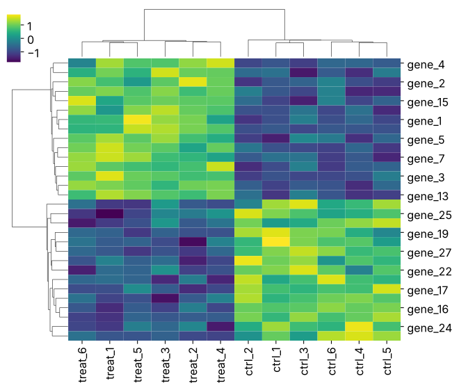
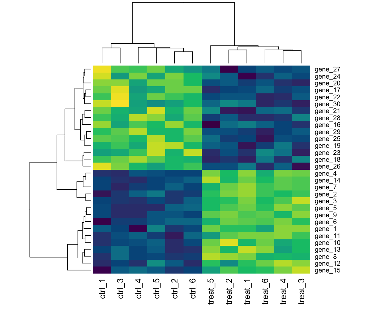
scale = "row"/z_score=0standardizes each gene, so the colors compare patterns, not absolute levels- The dendrograms are hierarchical clustering - both tools run it for you; richer R options:
pheatmap,ComplexHeatmap - The synthesis is the random-draws section at work:
rnorm()baselines plus shifted modules
Gallery 2: growth curves with ribbons
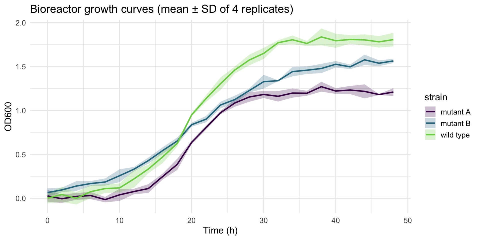
params <- tibble(strain = c("wild type", "mutant A", "mutant B"),
                 K = c(1.8, 1.2, 1.6),            # carrying capacity
                 r = c(0.25, 0.35, 0.15))         # growth rate
growth <- expand_grid(params, rep = 1:4, time = seq(0, 48, by = 2)) |>
  mutate(od = K / (1 + exp(-r * (time - 20))) + rnorm(n(), sd = 0.05))

growth |>
  group_by(strain, time) |>
  summarize(mean = mean(od), sd = sd(od), .groups = "drop") |>
  ggplot(aes(time, mean, color = strain, fill = strain)) +
  geom_ribbon(aes(ymin = mean - sd, ymax = mean + sd), alpha = 0.25, color = NA) +
  geom_line(linewidth = 1) +
  scale_color_viridis_d(end = 0.8) + scale_fill_viridis_d(end = 0.8) +
  labs(x = "Time (h)", y = "OD600",
       title = "Bioreactor growth curves (mean ± SD of 4 replicates)") +
  theme_minimal(base_size = 14)

ggsave("results/growth_curves.svg", width = 7, height = 5)
t = np.arange(0, 49, 2)
strains = {"wild type": (1.8, 0.25), "mutant A": (1.2, 0.35), "mutant B": (1.6, 0.15)}
fig, ax = plt.subplots()
for (name, (K, r)), c in zip(strains.items(), ["#440154", "#31688e", "#35b779"]):
reps = np.array([K / (1 + np.exp(-r * (t - 20))) + rng.normal(0, 0.05, len(t))
for _ in range(4)])
m, s = reps.mean(axis=0), reps.std(axis=0)
ax.plot(t, m, color=c, lw=2, label=name)
ax.fill_between(t, m - s, m + s, color=c, alpha=0.25)
ax.set(xlabel="Time (h)", ylabel="OD600")
ax.legend()
plt.savefig("results/growth_curves.svg")
plt.show()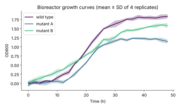
- The
group_by() |> summarize()+ ribbon pattern works for any repeated time course: sensor logs, qPCR curves, cyclic loading of a hydrogel - The synthesis itself is the random-draws section at work: a deterministic logistic curve plus
rnorm()noise
Gallery 3: dose-response curves
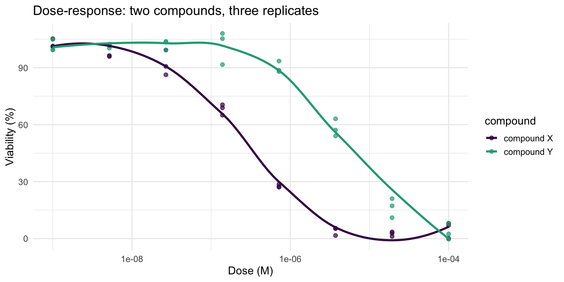
dr <- expand_grid(tibble(compound = c("compound X", "compound Y"),
                         ic50 = c(3e-7, 5e-6)),
                  rep = 1:3,
                  dose = 10^seq(-9, -4, length.out = 8)) |>
  mutate(viability = 100 / (1 + (dose / ic50)^1.2) + rnorm(n(), sd = 4))

ggplot(dr, aes(dose, viability, color = compound)) +
  geom_point(alpha = 0.7, size = 2) +
  geom_smooth(se = FALSE) +
  scale_x_log10() +
  scale_color_viridis_d(end = 0.6) +
  labs(x = "Dose (M)", y = "Viability (%)",
       title = "Dose-response: two compounds, three replicates") +
  theme_minimal(base_size = 14)

ggsave("results/dose_response.svg", width = 7, height = 5)
dose = np.logspace(-9, -4, 8)
fig, ax = plt.subplots()
for (name, ic50), c in zip({"compound X": 3e-7, "compound Y": 5e-6}.items(),
["#440154", "#35b779"]):
for _ in range(3):
viab = 100 / (1 + (dose / ic50) ** 1.2) + rng.normal(0, 4, len(dose))
ax.scatter(dose, viab, s=18, alpha=0.6, color=c)
grid = np.logspace(-9, -4, 200)
ax.plot(grid, 100 / (1 + (grid / ic50) ** 1.2), color=c, lw=2, label=name)
ax.set(xscale="log", xlabel="Dose (M)", ylabel="Viability (%)")
ax.legend()
plt.savefig("results/dose_response.svg")
plt.show()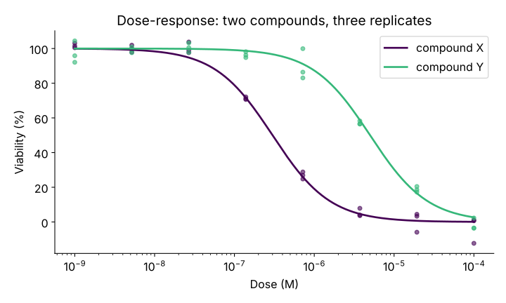
- A log-scaled x axis (
scale_x_log10()/xscale="log") is what makes dose-response curves readable - doses span five orders of magnitude geom_smooth()draws a data-driven trend; a real assay would fit a four-parameter logistic model (coming in the statistics sequence)
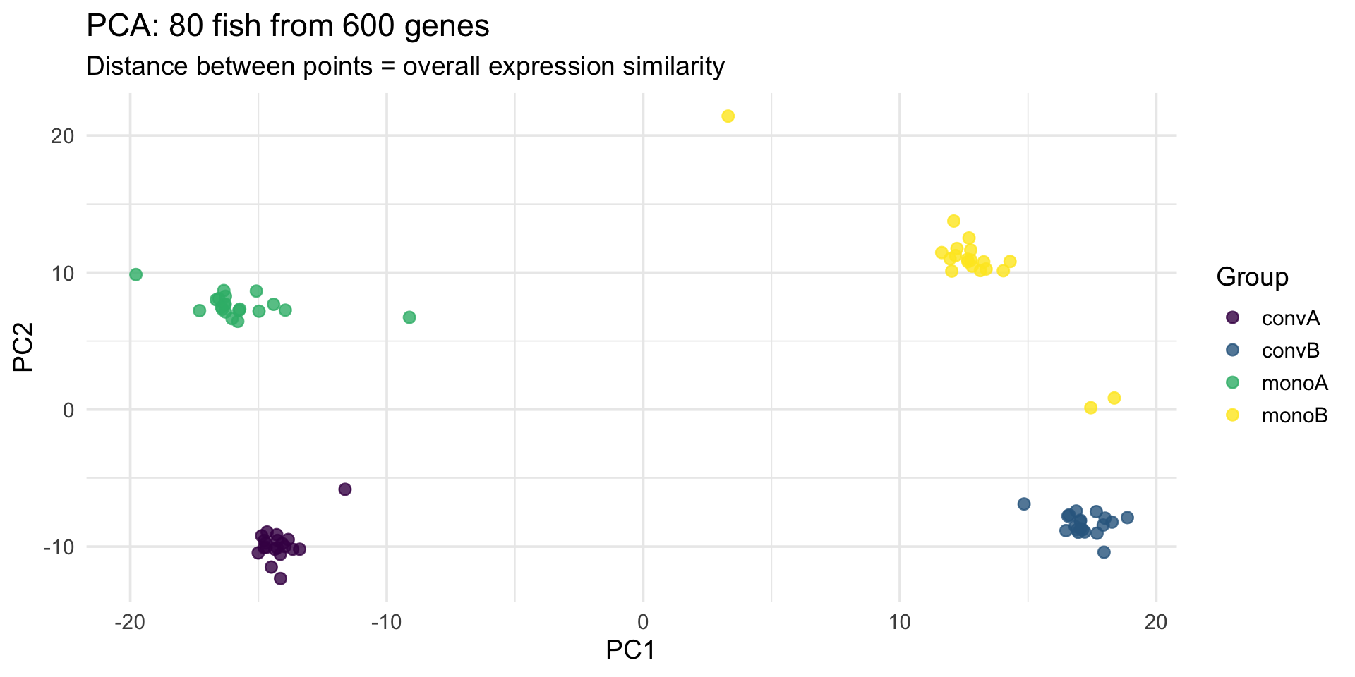
Gallery 4: PCA of the real stickleback fish
gene_mat <- stickle |> select(starts_with("Gene"))
pca <- prcomp(log1p(gene_mat), scale. = TRUE)     # log1p tames the counts

bind_cols(as_tibble(pca$x[, 1:2]),
          stickle |> select(geno_micro)) |>
  ggplot(aes(PC1, PC2, color = geno_micro)) +
  geom_point(size = 2.5, alpha = 0.8) +
  scale_color_viridis_d(name = "Group") +
  labs(title = "PCA: 80 fish from 600 genes",
       subtitle = "Distance between points = overall expression similarity") +
  theme_minimal(base_size = 14)

ggsave("results/pca_fish.svg", width = 7, height = 5)
from sklearn.decomposition import PCA
X = np.log1p(stickle[genes].to_numpy())
X = (X - X.mean(axis=0)) / X.std(axis=0) # like scale. = TRUE
scores = PCA(n_components=2).fit_transform(X)
fig, ax = plt.subplots()
for grp, c in zip(sorted(stickle["Geno&Micro"].unique()),
["#440154", "#31688e", "#35b779", "#fde725"]):
sel = stickle["Geno&Micro"] == grp
ax.scatter(scores[sel, 0], scores[sel, 1], s=30, alpha=0.8, color=c, label=grp)
ax.set(xlabel="PC1", ylabel="PC2", title="PCA of 80 fish from 600 genes")
ax.legend(title="Group")
plt.savefig("results/pca_fish.svg")
plt.show()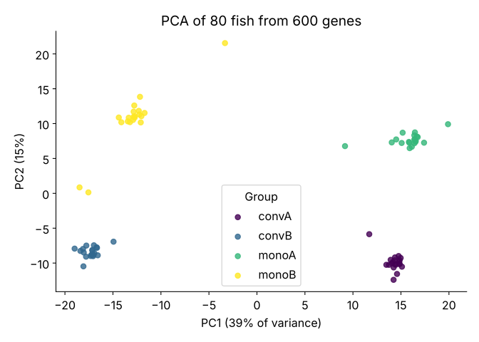
- PCA compresses 600 correlated gene columns into a few axes of maximal variation - the workhorse first look at any high-dimensional data set
- One
prcomp()call plus oneggplot()call; the groups separate because the biology is real