#!/usr/bin/env Rscript
# Script: plot_stickleback_boxplots.R
# Purpose: boxplots of total RNA-seq counts per group, written to an SVG

infile <- "data/Stickle_RNAseq.tsv"
if (!file.exists(infile)) {
  cat("Error: File", infile, "not found!\n")
  quit(status = 1)
}

stickle <- read.delim(infile, check.names = FALSE)  # keep the name "Geno&Micro"
genes   <- grep("^Gene", names(stickle))            # which columns are genes?
totals  <- rowSums(stickle[, genes])                # one number per fish
group   <- stickle[["Geno&Micro"]]

dir.create("results", showWarnings = FALSE)
svg("results/total_counts_by_group.svg", width = 7, height = 5)
boxplot(totals ~ group,
        xlab = "Genotype x microbiota group",
        ylab = "Total reads per fish",
        main = "Stickleback gut RNA-seq: total counts by group")
invisible(dev.off())    # close the file device, quietly
cat("Wrote results/total_counts_by_group.svg\n")Lecture 05
R and Python Fundamentals 1: Scripts, Variables, Types and Files
Bill Cresko
2026-10-26
Book reading for this lecture
The course book goes deeper on everything in this lecture. Read before or after class:
Python tutorial notebooks on the course website
- Prof. Parisa Hosseinzadeh teaches a parallel computational course, and we have posted her set of Python Jupyter notebooks on our Examples page
- Download them and run them cell by cell in Positron:
| Notebook | Topic |
|---|---|
s1_variables · s2_ConditionalStatements · s3_Loops |
variables and types · if/else · for/while |
s4_Functions · s5_Lists · s6_Dictionaries |
writing functions · lists and slicing · key-value storage |
s7_PandasDataframe · s8_PlottingData · s9_NumpyMatrices |
data frames · matplotlib/seaborn · numpy arrays |
Tip
- They are great self-study companions to L05-L06
s1ands5cover today’s material,s2-s4preview control flow and functions, ands7-s9preview the next two lectures.- New this week on the same page: two Lecture 05 notebooks (one R, one Python) with every example from today’s slides as runnable cells.
Goals for today
- Warm-up: last week’s stickleback plot, now as an R script and a Python script
- Why R and Python - same ideas, different syntax
- Variables, arithmetic, strings and vectors
- Types of data - and what R and Python call them
- Indexing rows, columns and cells of a data set
- Reading and writing files from a script (now opens L06)
grepand regular expressions, now in R and Python- Finale: write and run your own executable scripts
Warm-up - plot stickleback data
Last week’s job, two new languages
You have already piped the stickleback table through
grep,sedandawk, and in L03 you ran a first Python script on it.Here is that job again - read the data, total the counts per fish, draw boxplots by group - as an R script and a Python script that write the figure to an SVG file.
#!/usr/bin/env python3
# Script: plot_stickleback_boxplots.py
# Purpose: boxplots of total RNA-seq counts per group, written to an SVG

import sys
from pathlib import Path

import pandas as pd
import matplotlib
matplotlib.use("Agg")                 # draw straight to a file - no window
import matplotlib.pyplot as plt

infile = Path("data/Stickle_RNAseq.tsv")
if not infile.is_file():
    print(f"Error: File {infile} not found!")
    sys.exit(1)

stickle = pd.read_csv(infile, sep="\t")
genes   = [c for c in stickle.columns if c.startswith("Gene")]
totals  = pd.DataFrame({
    "Group": stickle["Geno&Micro"],
    "Total": stickle[genes].sum(axis=1),          # one number per fish
})

Path("results").mkdir(exist_ok=True)
totals.boxplot(column="Total", by="Group")
plt.suptitle("")                      # drop pandas' default super-title
plt.title("Stickleback gut RNA-seq: total counts by group")
plt.xlabel("Genotype x microbiota group")
plt.ylabel("Total reads per fish")
plt.savefig("results/total_counts_by_group.svg")  # .svg picks the format
print("Wrote results/total_counts_by_group.svg")
The figure both scripts write
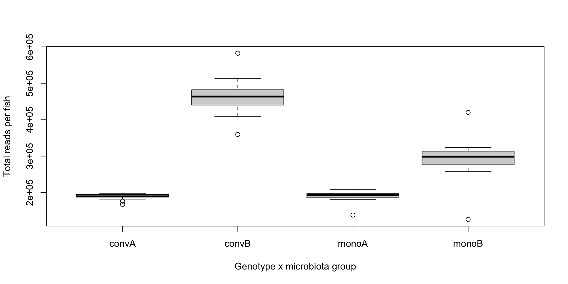
Figure 1: Total RNA-seq reads per fish in each genotype-by-microbiota group - the SVG written by both warm-up scripts
- An SVG is a vector figure: text-based, tiny, and it stays sharp at any zoom - open it in a browser, Illustrator or Inkscape
- Figure formats get their full story at the start of L06, in Reading and writing files
Running R and Python scripts from the shell
Rscriptruns the file top to bottom and prints only what youcat()orprint()- In Positron / VS Code: open the
.Rfile and pressCmd/Ctrl-Enterto send lines to the console
python3 script.pyruns the file top to bottom and prints only what youprint()- In Positron / VS Code: open the
.pyfile and pressCmd/Ctrl-Enter, or use the Run button - Keep project packages in a virtual environment:
python3 -m venv .venv && source .venv/bin/activate(environments get their full story in L09)
Tip
Both languages give a script an exit status (
quit(status = 1)/sys.exit(1)), so a shell pipeline or SLURM job can tell whether it succeeded - just likeexit 1in bash.You will write both of these scripts yourself in the finale, and in Lecture 08 we submit them to Talapas inside an
sbatchjob.
R and Python
Why use R?
- Good general scripting tool for statistics and mathematics
- Powerful and flexible and free
- Runs on all computer platforms
- New enhancements coming out all the time
- Superb data management & graphics capabilities
- Reproducibility - can keep your scripts to see exactly what was done
- You can write your own functions
- Lots of online help available
- Can use a nice IDE such as
Positron - Can embed your
Ranalyses in dynamic, polished files usingQuarto Markdown - Quarto Markdown can be reused for websites, papers, books, presentations…
Why use Python?
- A general-purpose language that is also excellent for data analysis (
pandas,numpy,matplotlib,scipy) - The language of machine learning, image analysis and instrument control (
scikit-learn,PyTorch,scikit-image) - Free, open source, runs everywhere - including Talapas (
module load python3) - Huge ecosystem:
pip installgives you access to >500,000 packages on PyPI;condaadds compiled scientific tools - Readable syntax; indentation is the structure of the code
- Runs as scripts (
python3 script.py), interactively (REPL / IPython), in Jupyter notebooks, and in Quarto{python}chunks - Same IDE: Positron (and VS Code) runs R and Python side by side
Tip
You do not have to choose. Most computational biologists use both:
R for statistics and figures
Python for pipelines, images and machine learning.
This lecture shows every idea in both languages - use the tabs.
R vs Python: same ideas, different syntax
| Idea | R | Python |
|---|---|---|
| Assignment | x <- 5 |
x = 5 |
| Counting starts at | 1: x[1] is the first element |
0: x[0] is the first element |
| Last element | x[length(x)]; x[-1] drops the first |
x[-1] is the last |
| Sequence of values | vector c(1, 2, 3) |
list [1, 2, 3] or numpy array np.array([1, 2, 3]) |
| Vector arithmetic | x^2 on any vector |
x**2 only on a numpy array (a list needs a loop) |
| Table of data | data.frame / tibble |
pandas DataFrame |
| Load a package | library(dplyr) |
import pandas as pd |
| Install a package | install.packages("dplyr") |
pip install pandas |
| Chain steps | pipe x |> f() |> g() |
method chaining x.f().g() |
| Blocks | curly braces { } |
indentation (4 spaces) |
| Missing value | NA |
None, float("nan"), pd.NA |
| Help | ?mean |
help(statistics.mean) or mean? in Jupyter |
R and Python syntax
Every example in this section and the next two is a runnable cell in the two companion notebooks on the Examples page:
Lecture05_R_fundamentals.ipynbandLecture05_Python_fundamentals.ipynb.Download them, open them in Positron, and run along.
Two topics live only in the notebooks - working with strings (
paste0,sprintf/ f-strings, slicing) and managing your workspace (ls(),rm()/del,%whos) - so be sure to run those cells too.
The basics: arithmetic
- Commands can be submitted through the terminal, console or scripts (R:
R/Rscript; Python:python3/python3 script.py) - Notice on these slides I’m evaluating the code chunks and showing output
- Also notice that both languages follow the normal priority of mathematical evaluation
- Careful: exponent is
^in R but**in Python (^in Python is bitwise XOR!)
Assigning variables
- Assign values with
<-in R and=in Python - R also accepts
=for assignment, but course (and community) style is<- - Python can assign several variables at once:
a, b = 1, 2
Arithmetic operations on functions
- Arithmetic operations can be performed easily on functions as well as numbers.
- Try the following, and then your own.
- Note that the last of these -
log- is a built in function ofR, and therefore the object of the function needs to be put in parentheses - In Python,
loglives in themathmodule, so weimport mathonce and callmath.log(x)(numpyhasnp.log()for whole arrays) - These parentheses will be important, and we’ll come back to them later when we add arguments after the object in the parentheses
- The outcome of calculations can be assigned to new variables as well, and the results can be checked using the ‘print’ command
Arithmetic operations on functions
Comparisons and logical values
- Comparisons ask questions about values and return a logical (R) or bool (Python) - the foundation of filtering and indexing later today
- R spells the logical values
TRUE/FALSE; Python capitalizes only the first letter:True/False - R uses the symbols
&,|,!; Python uses the wordsand,or,not(the symbols&and|are reserved for element-wise work on numpy arrays and pandas columns) - Much more on logical operators and filtering in L06 and its self-study notebooks
STRINGS
- Variables and operations can be performed on characters as well
- Note that characters need to be set off by quotation marks to differentiate them from numbers
- The
cstands forconcatenate; in Python square brackets[ ]build a list - Note that we are using the same variable names as we did previously, which means that we’re overwriting our previous assignment
- A good rule of thumb is to use new names for each variable, and make them short but still descriptive
STRINGS
VECTORS
- In general
Rthinks in terms of vectors (a list of characters, factors or numerical values). - It will benefit any
Ruser to try to write programs with that in mind, as it will simplify most things. - Vectors can be assigned directly using the
c()function and then entering the exact values. - Python has lists (
[ ]) for any collection, and numpy arrays (np.array()) when you want R-style vector math x^2squares every element of an R vector; in Python that only works on a numpy array - a list needs a loop or a list comprehension
VECTORS
Creating vectors
- Typing vectors in by hand is a drag - use generating functions instead:
seq()andrep()in R;range(),np.arange(),np.linspace()in Python - Try the examples and vary the arguments - can you work out what each one does?
  [1]  0.0  0.1  0.2  0.3  0.4  0.5  0.6  0.7  0.8  0.9  1.0  1.1  1.2  1.3  1.4
 [16]  1.5  1.6  1.7  1.8  1.9  2.0  2.1  2.2  2.3  2.4  2.5  2.6  2.7  2.8  2.9
 [31]  3.0  3.1  3.2  3.3  3.4  3.5  3.6  3.7  3.8  3.9  4.0  4.1  4.2  4.3  4.4
 [46]  4.5  4.6  4.7  4.8  4.9  5.0  5.1  5.2  5.3  5.4  5.5  5.6  5.7  5.8  5.9
 [61]  6.0  6.1  6.2  6.3  6.4  6.5  6.6  6.7  6.8  6.9  7.0  7.1  7.2  7.3  7.4
 [76]  7.5  7.6  7.7  7.8  7.9  8.0  8.1  8.2  8.3  8.4  8.5  8.6  8.7  8.8  8.9
[91] 9.0 9.1 9.2 9.3 9.4 9.5 9.6 9.7 9.8 9.9 10.0 [1] 100.00 98.01 96.04 94.09 92.16 90.25 88.36 86.49 84.64 82.81
[11] 81.00 79.21 77.44 75.69 73.96 72.25 70.56 68.89 67.24 65.61
[21] 64.00 62.41 60.84 59.29 57.76 56.25 54.76 53.29 51.84 50.41
[31] 49.00 47.61 46.24 44.89 43.56 42.25 40.96 39.69 38.44 37.21
[41] 36.00 34.81 33.64 32.49 31.36 30.25 29.16 28.09 27.04 26.01
[51] 25.00 24.01 23.04 22.09 21.16 20.25 19.36 18.49 17.64 16.81
[61] 16.00 15.21 14.44 13.69 12.96 12.25 11.56 10.89 10.24 9.61
[71] 9.00 8.41 7.84 7.29 6.76 6.25 5.76 5.29 4.84 4.41
[81] 4.00 3.61 3.24 2.89 2.56 2.25 1.96 1.69 1.44 1.21
[91] 1.00 0.81 0.64 0.49 0.36 0.25 0.16 0.09 0.04 0.01
[101] 0.00[1] "A" "B" "A" "B" "A" "B"[1] "A" "A" "A" "B" "B" "B"import numpy as np
seq_1 = np.linspace(0.0, 10.0, 101) # 101 points from 0 to 10 (step 0.1)
print(seq_1)
# [ 0. 0.1 0.2 ... 9.8 9.9 10. ]
seq_2 = np.linspace(10.0, 0.0, 101)
seq_square = seq_2 * seq_2 # element-wise ...
seq_square_new = seq_2**2 # ... same result
print(seq_square_new)
# [100. 98.01 96.04 ... 0.04 0.01 0. ]
list(range(10)) # integers 0, 1, ..., 9 (start defaults to 0; stop excluded!)
np.tile(["A", "B"], 3) # like rep(..., times = 3)
# ['A' 'B' 'A' 'B' 'A' 'B']
np.repeat(["A", "B"], 3) # like rep(..., each = 3)
# ['A' 'A' 'A' 'B' 'B' 'B']Basic Statistics
- Many functions exist to operate on vectors.
- Combine these with your previous variable to see what happens.
- Also, try to find other functions (e.g. standard deviation).
import numpy as np

x.mean()                     # or np.mean(x)
np.median(x)
x.var(ddof=1)                # sample variance, like R's var()
np.log(x)                    # natural log, element-wise
np.sqrt(x)
x.sum()                      # sum(x) also works
len(x)                       # length(x)
rng = np.random.default_rng(2026)         # a seeded random generator (like set.seed)
rng.choice(x, size=len(x), replace=True) # sample with replacement- Notice that the last function (
sample) has an argument (replace=T); in Python the generator’srng.choice()samples with replacement whenreplace=True, andsize=sets how many - the samedefault_rng()generator powers all the random sampling in L06 - Python functions come in two flavours:
np.median(x)(function) andx.mean()(a method attached to the array) - Arguments simply modify or direct the function in some way
- There are many arguments for each function, some of which are defaults
Getting Help
- Getting Help on any function is very easy - just type a question mark and the name of the function (R), or
help(function)in Python. - There are functions for just about anything within
Rand it is easy enough to write your own functions if none already exist to do what you want to do. - In general, function calls have a simple structure: a function name, a set of parentheses and an optional set of parameters to send to the function.
- Help pages exist for all functions that, at a minimum, explain what parameters exist for the function.
- Help can be accessed a few ways - try them :
Getting Help
import numpy as np, inspect

help(np.mean)                # full documentation, any Python
np.mean?                     # short help - IPython, Jupyter, Positron only
np.mean??                    # ... plus the source code
dir(np)                      # list everything inside a module
[n for n in dir(np) if "mean" in n]   # like apropos("mean")
inspect.signature(np.mean) # like args(mean)Data types in R and Python
Scales of measurement
| Scale | What it is | Example | Typical computer type |
|---|---|---|---|
| Nominal (categorical) | Unordered labels | genotype A / B; apples, oranges | character or factor |
| Ordinal (categorical) | Ordered labels | small < medium < large | ordered factor |
| Discrete (quantitative) | Whole-number counts | RNA-seq reads per gene | integer |
| Continuous (quantitative) | Measurements | mass (kg), length (mm) | double / float |
- Among continuous scales:
- a ratio scale has a true zero (mass, length, counts);
- an interval scale does not (temperature in °C, calendar year)
Factoris R’s special type for categorical variables - we will explore it more later
The same types, two sets of names
| What it holds | R (tibble code) | Python | Example |
|---|---|---|---|
| TRUE / FALSE | logical (lgl) |
bool |
TRUE / True |
| Whole numbers | integer (int) |
int |
3L / 3 |
| Real numbers | double (dbl) |
float |
3.0, 2.5e-3 |
| Text | character (chr) |
str |
"low" |
| Categories | factor (fctr) |
pandas.Categorical |
factor(c("low","high")) |
| Dates / date-times | date / dttm |
datetime.date / datetime.datetime |
as.Date("2026-11-09") |
- Integer and double vectors are known collectively as numeric vectors; in
Rnumbers are doubles by default - Python keeps
intandfloatstrictly apart:7 / 2is3.5(always a float)7 // 2is3(integer division)7 % 2is the remainder1
- R’s integer division and remainder are
%/%and%%
Checking what type you have
class()/type()answer “what is this?”;str()in R and.dtype/.info()in pandas summarize bigger structures- A numpy array or pandas column has one dtype shared by every value - just like an R vector
Converting between types
- The two languages fail differently:
- R converts the unconvertible to
NAwith a warning and keeps going - Python raises an error and stops
- R converts the unconvertible to
- Both behaviors bite: check for
NAafter converting in R; wrap risky conversions intry/exceptin Python (Ch. 12)
One type per vector: coercion
- An R vector holds exactly one type - mix types and R silently coerces everything to the most flexible one: logical → integer → double → character
- Watch for this when reading data: one stray character in a column of numbers turns the whole column into strings
- A pandas column that mixes types gets dtype
object- slow and error-prone; the fix is cleaning the data, not ignoring it
Special values: missing, impossible and infinite
| Meaning | R | Python / pandas |
|---|---|---|
| Missing value | NA |
None, np.nan, pd.NA |
Not a number (e.g. 0/0) |
NaN |
float("nan"), np.nan |
Infinity (e.g. 1/0) |
Inf, -Inf |
math.inf, np.inf |
| No object at all | NULL |
None |
- Logical vectors can take exactly three values:
TRUE,FALSEandNA; doubles addNaN,Infand-Inf - Mind the opposite defaults: R keeps
NAunless you sayna.rm = TRUE; pandas skips missing values unless you sayskipna=False
Beyond vectors: lists and dictionaries
- A vector or array holds many values of one type; a list (R) or dictionary (Python) holds anything, with a name for each element
- Why this matters next: a data frame is a list of equal-length vectors - one name per column, one type per column; pandas builds a
DataFramefrom a dictionary of columns the same way - Python also has tuples (
(1, 2), immutable) and sets ({1, 2}, unique values) - Parisa’ss5ands6notebooks work through all four
Indexing
Indexing vectors and lists
[1] 2[1] 2 4[1] 3 4 2 [1] 3 4 2 1 2 4 5 10 8 9[1] 5 10 8 9import numpy as np
x = np.array([2, 3, 4, 2, 1, 2, 4, 5, 10, 8, 9])
x[0] # the FIRST element - Python counts from 0
# 2
x[[0, 2]] # elements at positions 0 and 2
# [2 4]
x[1:4] # positions 1, 2, 3 - the stop position is EXCLUDED
# [3 4 2]
x[-1] # the LAST element (negative = count from the end)
# 9
x[x > 4] # logical (boolean) indexing, exactly like R
# [ 5 10 8 9]- The same
[ ]syntax, two opposite conventions: R is 1-based and inclusive, Python is 0-based and stop-excluded - Negative numbers drop elements in R but count from the end in Python - the classic cross-language bug
- Logical indexing (
x[x > 4]) is identical in both - and it is the idea behind filtering tables, next
Indexing a data set: columns
First read the stickleback table (full story in the next section), then pull out columns:
[1] "A" "A" "A" "A" "A" "A"[1] "convA" "convA" "convA" "convA" "convA" "convA" Individual Genotype
1 AC1 A
2 AC2 A
3 AC3 Aimport pandas as pd
stickle = pd.read_csv("../Data_Folder/Stickle_RNAseq.tsv", sep="\t")
stickle["Genotype"].head() # one set of brackets -> a Series (a column)
# 0 A, 1 A, 2 A, ...
stickle["Geno&Micro"].head() # any column name works in brackets
stickle[["Individual", "Genotype"]].head(3) # a LIST of names -> a DataFrame- One column:
stickle$Genotype(R) ↔︎stickle["Genotype"](Python) $only works for simple names;[[ ]](R) and[" "](Python) work for any name - like our awkwardGeno&Micro- Single brackets with a list of names return a smaller table in both languages
Indexing a data set: rows and single cells
Both languages use table[row, column] - the differences are the starting number and labels vs positions:
  Individual Genotype   Microbiota Geno&Micro
1 AC1 A conventional convA Individual Genotype
1 AC1 A
2 AC2 A
3 AC3 A[1] "A"[1] "A"- R has one bracket for both jobs; pandas splits them:
.loc[ ]for labels,.iloc[ ]for positions - Careful:
.loc[0:2]includes both ends (label slicing), while.iloc[0:2]excludes the stop - position slicing behaves like the rest of Python
Indexing a data set: rows by condition
The logical indexing from vectors scales straight up to tables - keep the rows where this is TRUE:
[1] 40 Individual Genotype Microbiota Geno&Micro
61 BM1 B mono monoB
62 BM2 B mono monoB
63 BM3 B mono monoBTip
This is
grepfor tables: in L04 you kept matching lines withgrep mono;Today you keep matching rows with a logical test.
The tidyverse (
filter(), L06) and pandas (.query()) wrap this same idea in friendlier syntax.
grep and regular expressions in R and Python
The same patterns, new functions
| Job | Shell (L04) | R | Python (import re) |
|---|---|---|---|
| Which elements match? | grep |
grepl() (TRUE/FALSE), grep() (positions) |
re.search() |
| Pull out the match | grep -o |
regmatches() + gregexpr() |
re.findall() |
| Substitute | sed 's/a/b/' |
sub() (first), gsub() (all) |
re.sub() |
| Split on a pattern | awk -F |
strsplit() |
re.split() |
- The patterns themselves are the same ones you learned in L04:
^start,$end,[ACGT]classes,{3}counts,( | )alternatives - Two escaping dialects:
- R needs a double backslash (
"\\d"for a digit) - Python uses raw strings (
r"\d") - always write Python patterns with therprefix
- R needs a double backslash (
- The tidyverse’s
stringr(str_detect(),str_replace(), …) wraps R’s functions with consistent names
Regular expressions on the stickleback table
[1] 600[1] "AC1" "AC11" "AM1" "AM11" "BC1" "BC11" "BM1" "BM11"[1] "G1" "G2" "G3" "G4"[1] "c" "o" "n" "v" "A"import re
[c for c in stickle.columns if re.search(r"^Gene", c)][:3] # gene columns
# ['Gene1', 'Gene2', 'Gene3']
stickle["Individual"][stickle["Individual"].str.contains(r"1$")]
# the pandas .str methods apply a regex down a whole column
[re.sub(r"^Gene", "G", c) for c in stickle.columns[4:8]]
# ['G1', 'G2', 'G3', 'G4']
re.split(r"", "convA") # and re.findall(r"[A-Z]", "convA") pulls out ['A']grepl()onnames(stickle)is exactly how the warm-up script found the 600 gene columns- In pandas, the
.straccessor (.str.contains(),.str.replace(),.str.extract()) runs a regex down an entire column at once
The L04 fasta_stats bash script in R and Python
#!/usr/bin/env Rscript
# Script: fasta_stats.R
# Purpose: Calculate basic statistics for a FASTA file

args <- commandArgs(trailingOnly = TRUE)     # like $1 $2 ... in bash
if (length(args) != 1) {
  cat("Usage: Rscript fasta_stats.R sequences.fasta\n")
  quit(status = 1)
}
input <- args[1]
if (!file.exists(input)) {
  cat("Error: File", input, "not found!\n")
  quit(status = 1)
}

lines   <- readLines(input)
headers <- grepl("^>", lines)                # TRUE for header lines
seq     <- paste(lines[!headers], collapse = "")

cat("=== FASTA Statistics for", input, "===\n")
cat("Number of sequences:", sum(headers), "\n")
cat("Total length:", nchar(seq), "bp\n")
cat("Average length:", nchar(seq) / sum(headers), "bp\n")
n_count <- sum(strsplit(seq, "")[[1]] %in% c("N", "n"))
cat("N bases:", n_count, "\n")
gc <- sum(strsplit(toupper(seq), "")[[1]] %in% c("G", "C"))
cat("GC content:", round(100 * gc / nchar(seq), 1), "%\n")
orfs <- regmatches(seq, gregexpr("ATG([ACGT]{3}){20,}(TAA|TAG|TGA)", seq))[[1]]
cat("ORF-like stretches:", length(orfs), "\n")
#!/usr/bin/env python3
# Script: fasta_stats.py
# Purpose: Calculate basic statistics for a FASTA file
import re
import sys
from pathlib import Path
if len(sys.argv) != 2: # sys.argv[0] is the script name, like $0
print("Usage: python3 fasta_stats.py sequences.fasta")
sys.exit(1)
input_file = Path(sys.argv[1])
if not input_file.is_file():
print(f"Error: File {input_file} not found!")
sys.exit(1)
lines = input_file.read_text().splitlines()
headers = [line for line in lines if line.startswith(">")]
seq = "".join(line for line in lines if not line.startswith(">"))
print(f"=== FASTA Statistics for {input_file} ===")
print(f"Number of sequences: {len(headers)}")
print(f"Total length: {len(seq)} bp")
print(f"Average length: {len(seq) / len(headers):.1f} bp")
n_count = seq.count("N") + seq.count("n")
print(f"N bases: {n_count}")
gc = seq.upper().count("G") + seq.upper().count("C")
print(f"GC content: {100 * gc / len(seq):.1f}%")
orfs = re.findall(r"ATG(?:[ACGT]{3}){20,}(?:TAA|TAG|TGA)", seq)
print(f"ORF-like stretches: {len(orfs)}")Finale: write your own executable R and Python scripts
Anatomy of an executable script
| Ingredient | bash (L02-L04) | R | Python |
|---|---|---|---|
| Shebang (line 1) | #!/bin/bash |
#!/usr/bin/env Rscript |
#!/usr/bin/env python3 |
| Make it executable | chmod +x name.sh |
chmod +x name.R |
chmod +x name.py |
| Run it | ./name.sh |
./name.R (or Rscript name.R) |
./name.py (or python3 name.py) |
| Arguments | $1, $2 |
commandArgs(trailingOnly = TRUE) |
sys.argv[1:] |
echo |
cat() |
print() |
|
| Fail loudly | exit 1 |
quit(status = 1) |
sys.exit(1) |
- The shell does not care what language is inside - the shebang tells it which interpreter to hand the file to
- That is why these scripts drop into any pipeline,
cronjob orsbatchsubmission exactly like your week-2 shell scripts
Your turn 1: the box-plot script
Write the warm-up script yourself in the language you know less well (or both!):
- In Positron, create
scripts/plot_stickleback_boxplots.Ror.pyin your course project (~/projects/comptools) - type it in; no pasting - Add the shebang, read
data/Stickle_RNAseq.tsv, total the gene columns, draw the boxplots, writeresults/total_counts_by_group.svg chmod +xit and run it from the project root; open the SVG in your browser- Modify it: plot
Gene1instead of the totals; group byGenotypealone; write a PNG at 300 dpi alongside the SVG
Working versions of both scripts are on the Examples page - but only look after your own runs.
Your turn 2: fasta_stats, the regex one
Now the harder one, with command-line arguments and regular expressions:
- Write
scripts/fasta_stats.Rorscripts/fasta_stats.py - Test on L04’s small file first, then the real one:
- Check yourself against last week: the bash and R/Python versions should agree
- Stretch goals: report the longest ORF-like stretch; print a per-sequence table (name, length, GC) instead of totals; make the ORF minimum length (
{20,}) a second command-line argument
Summary
- R and Python share the ideas - variables, vectors, types, indexing, files - and differ in spelling:
<-vs=,^vs**, 1-based vs 0-based,TRUEvsTrue - A script is a text file plus a shebang,
chmod +x, arguments and an exit status - in any language - Every vector/column has one type; know
class()/type(), convert deliberately, and respectNA/NaN(and the oppositena.rm/skipnadefaults) - Indexing:
x[i],table[row, col],$/[[ ]],.loc/.iloc- and logical tests select rows likegrepselects lines - Regular expressions moved with you: the L04 patterns now run inside
grepl()/gsub()andre.findall()/re.sub() - Next week (L06): reading and writing files, then data frames in earnest - distributions, summaries and real figures from the stickleback table
BioE Computational Tools 2026 - Knight Campus
Comments, names and style
#and run to the end of the line - in bash, R and PythonWeight,weightandWEIGHTare three different names_(and.in R); must not start with a digitsnake_case, short but descriptive -mean_gc,n_fish,total_reads