Lecture 07
Reproducible Documents and AI-Assisted Coding
2026-11-09
Book reading for this lecture
The course book goes deeper on everything in this lecture. Read before or after class:
Goals for today
- Why literate programming is the backbone of reproducible, FAIR science
- The anatomy of a Quarto document - YAML, prose, and code chunks (R and Python)
- Typesetting mathematics with LaTeX
- Inserting Citations from a
.bibfile - Three live demos, one per output format: slides, a manuscript PDF, and a website
- AI-assisted coding - the core principles
Tip
The three demo files are yours to download, break, and reuse: Example Files, Week 7.
Literate programming and reproducible science
Your paper and your analysis drift apart
- The classic workflow:
- analyze over here (scripts, console)
- write over there (Word)
- hand-carry numbers and figures between them
- Every revision re-opens the gap:
- figure version five in a version-three draft
- a mean in the text the code no longer produces
- methods that describe last month’s analysis
- Scientific bugs are usually silent - nothing crashes when the pasted number is stale
- An analysis you cannot regenerate is one you cannot defend - to reviewers, collaborators, or yourself in six months
Literate programming: the document is the analysis
“Instead of imagining that our main task is to instruct a computer what to do, let us concentrate rather on explaining to human beings what we want a computer to do.” - Donald Knuth, Literate Programming (1984)
- One plain-text document holds the prose, the code, and the results - rendering re-runs everything from data to figures
- The numbers in your sentences are computed, not typed, so they can never disagree with your data
- Your methods become self-documenting so inconsistencies between what you say and what you do become visible
- We already do this - our lab notebook templates, the companion notebooks, this very slide deck and the course book are all Quarto
Reproducibility has a policy behind it: FAIR
- Funders (including NIH and NSF) expect research outputs to be FAIR:
- Findable - deposited somewhere with a persistent identifier, not “available upon request”
- Accessible - retrievable by standard tools, no special software or permission maze
- Interoperable - open, documented formats (tidy
.tsvand.qmd) - Reusable - enough documentation and provenance that someone else can use it
- Literate documents are FAIR practice
- plain text any tool can read
- methods that travel with the analysis
- one source anyone can re-run
- The arc of the rest of the course:
- today the documents
- → Week 8 sharing it all on GitHub
- → Weeks 9 & 10 the environments and Talapas
Quarto Markdown
Markdown: formatting in plain text
Markdown is a lightweight language: you type plain text with a few marks, and a renderer turns it into formatted output.
You type:
Headers mark the document’s structure - one # per level:
Markdown: lists, quotes, tables, and images
You type:
You get:
- stickleback
- zebrafish
- AB strain
- collect
- measure
- analyze
Form follows function.
A table is rows of |-separated cells; the dashed line separates the header from the body (a colon on the dashes sets alignment):
| Genotype | n | Mean |
|---|---|---|
| A | 40 | 11.2 |
| B | 40 | 14.6 |
An image is one line - a path or URL, with optional sizing:
Quarto Markdown
Quarto extends Markdown into a scientific publishing system.
A
.qmdfile isMarkdownplus three ingredients:
- A YAML header - document settings and metadata at the top
- Executable code chunks - R or Python that runs when the document renders
- Scholarly machinery - callouts, cross-references, LaTeX math, and citations
One
.qmdsource renders to HTML, PDF, Word, slides, websites, and booksThis slide deck, the course site, and the course book are all Quarto.
Ingredient 1: the YAML header
- The
---fences mark it off at the very top - Inside the YAML header is
key: valuepairs - It controls the whole document:
format:- picks the output (
html,pdf,docx,revealjs, …)
- picks the output (
- Options for a format nest beneath it, and
execute:- sets defaults for every code chunk:
Ingredient 2: Markdown prose between the chunks
- Everything from the last two slides works unchanged - headings, emphasis, lists, images
- The document reads as a narrative with the analysis embedded at the right moments
- This is literate programming
- Headings organize the output and your thinking: Methods, Results, etc….
Ingredient 3: executable code chunks
- Three back ticks fence a chunk
{r}runs it through knitr{python}through Jupyter
- Everything else about the chunk - options, labels, captions - is identical in both languages
- Mixing R and Python in one file works too (via the R package
reticulate) - details in Ch. 16
Chunk options: the hash-pipe #|
Options go inside the chunk, one per line - identical in every language:
| Option | Effect |
|---|---|
echo: false |
Run the code, hide the code (manuscripts!) |
eval: false |
Show the code, don’t run it |
include: false |
Run it, show nothing (setup chunks) |
fig-cap: |
Figure caption |
label: fig-... |
Makes the figure numbered and referenceable |
Tip
Set document-wide defaults in the YAML under
execute:Override chunk by chunk only where needed.
Inline code so sentences don’t go stale
- Renders as:
“We measured 600 genes in 80 fish (Figure 1).”
- Re-run with more fish next month, or add a figure
- the sentence updates itself
- the figures are re-numbered automatically
- This is a big practical win of literate programming
Callouts: boxes that organize your reader’s attention
You type:
You get:
Save your eyes
Five types: note, tip, warning, important, caution.
Warning
This step overwrites results/.
Cross-references: label it once, @ it anywhere
Label a figure, table, equation, or section; reference it with @; Quarto numbers everything, and renumbers on every render:
| Type | Label | Reference |
|---|---|---|
| Figure | #| label: fig-name or {#fig-name} |
@fig-name |
| Table | #| label: tbl-name or {#tbl-name} |
@tbl-name |
| Equation | $$ ... $$ {#eq-name} |
@eq-name |
| Section | ## Heading {#sec-name} |
@sec-name |
You type:
You get - a live, clickable reference to a figure that sits several slides ahead:
The render pipeline (Figure 1) runs your code every time.
Mathematics with LaTeX
Inline math: a single pair of $
LaTeX notation dropped between $ signs flows with the sentence:
| You type | You get |
|---|---|
$\sigma = E\varepsilon$ |
\(\sigma = E\varepsilon\) |
$\bar{x} \pm 1.96\, s/\sqrt{n}$ |
\(\bar{x} \pm 1.96\, s/\sqrt{n}\) |
$\mu = 2.5\ \mathrm{kPa}$ |
\(\mu = 2.5\ \mathrm{kPa}\) |
$H_0\!: \beta_1 = 0$ |
\(H_0\!: \beta_1 = 0\) |
- Subscripts with
_, superscripts with^, Greek letters by name (\sigma,\mu,\beta) - Works identically in HTML, PDF, Word, and slides
Display math: a double pair of $$
A $$ pair puts the expression on its own centered line:
\[Pr(Y=r) = \frac{e^{-\mu}\mu^r}{r!}\]
\[f(x) = \frac{1}{\sigma\sqrt{2\pi}} \, e^{-\frac{(x-\mu)^2}{2\sigma^2}}\]
\[\iint xy^2 \, dx \, dy = \frac{1}{6}x^2y^3\]
Numbered equations are cross-references too
You type (the {#eq-...} label sits on the same line as the closing $$):
You get:
\[ \mathrm{SE} = \frac{s}{\sqrt{n}} \tag{1}\]
The standard error (Equation 1) shrinks with sample size.
Citations
The reference database: a .bib file
BibTeX is a plain-text database - one entry per source, each with a citation key:
Wire it up in the YAML header:
- Zotero exports BibTeX directly
- Google Scholar’s “Cite” button offers an entry for any paper
- Keep one
.bibper project and let it grow - Swap the
.cslfile and every citation re-styles itself for a different journal
Citing with @key - and what it renders
You type:
You get (these are real citations - this deck has its own .bib file):
Knuth introduced literate programming (Knuth 1984). Knuth (1984) argued that programs are written for people. Research outputs should be FAIR (Wilkinson et al. 2016; Knuth 1984).
And Quarto builds the reference list for free, wherever you put a #refs div:
>
Rendering: one source, many outputs
What happens when you press render
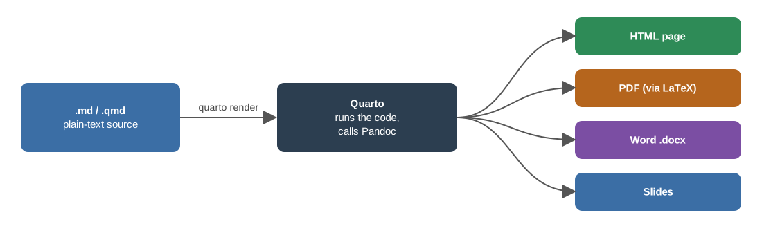
Figure 1: The render pipeline: Quarto runs the code (knitr for R, Jupyter for Python), weaves the results into the Markdown, and hands the whole thing to Pandoc to produce the output format.
- The code runs every time, so figures, tables, and inline numbers can never drift from the data
- This figure is
@fig-pipeline- the cross-reference you clicked three sections ago
Rendering commands
quarto render report.qmd              # the format named in the YAML
quarto render report.qmd --to pdf     # override: PDF (needs TinyTeX, installed once)
quarto render report.qmd --to docx    # override: Word
quarto preview report.qmd             # live preview - re-renders every time you save
quarto render # render a whole project or website- In Positron:
- the Preview button, or
Cmd/Ctrl + Shift + K - Or use the
quarto previewandquarto rendercommands in the terminal
- the Preview button, or
quarto previewis the one to use while writing- it opens the document beside your editor
- refreshes on every save
- PDF goes through LaTeX - install once with
quarto install tinytex, then forget it’s there - Emailing a report?
- Set
embed-resources: trueunderformat: html: - images, CSS, and JS are bundled into one self-contained
.htmlfile that travels on its own
- Set
One source, several formats
List several formats in the YAML and render them all at once:
| Output type | Formats |
|---|---|
| Documents | HTML, PDF (via LaTeX), Word |
| Presentations | RevealJS (these slides!), PowerPoint, Beamer |
| Websites and books | HTML (all of our class material!) |
Three demos with the same skeleton, three outputs
Demo 1: slides (example_slides.qmd)
format: revealjs - a deck like this one, from one .qmd.
Watch for:
##= new slide,#= section divider::: incrementaland. . .to reveal content stepwise- Two-column layouts, executed R chunks, stepwise code highlighting
- Tabsets, callouts, and math on slides
- Speaker notes (press S) and the overview (press O)
Demo 2: a manuscript (example_manuscript.qmd)
format: pdf - a Science/Nature-style article, LaTeX without writing LaTeX.
Watch for:
- Scholarly YAML: authors, affiliations, ORCID, corresponding author, abstract, keywords
echo: false- readers see results, never code- Inline and display math, numbered equations, and
@fig-/@tbl-/@eq-/@sec-cross-references throughout - Superscript citations from
example_manuscript.bib+nature.csl, reference list built for free - Companion files travel with the source:
.bib,.csl,title.tex
Important
Your term project report should start from this skeleton - create the .qmd this week.
Demo 3: a website (example_website.zip)
A folder, not a file - _quarto.yml turns it into a project; every .qmd becomes a page.
Watch for:
_quarto.yml: the navbar, theme, andoutput-dir: docs- An
about:landing page template for your photo + links quarto previewfor a live local version while you edit- Research / publications / CV pages - a complete academic site for a graduate student
Tip
Keep your copy. In Week 8 we push exactly this folder to GitHub and flip on GitHub Pages - it becomes your-username.github.io, for free.
AI-assisted coding
“Vibe coding” and why it can fail in science
- A large language model (LLM) predicts the most plausible next text - including code
- Vibe coding = describe, accept, run, paste the error, repeat - without reading the code
- Fun for a weekend project; a problem for science:
- you have to defend every result
- scientific bugs are usually silent (wrong number, no crash)
- you stop learning
- Here’s a different approach:
- keep the speed, drop the blindness
- the assistant writes, you read,
- a tiny test decides
The loop
- Describe the goal precisely - language, versions, sample input, expected output
- Get code
- READ it - every line; look up anything you don’t recognize
- Run it on a tiny test you can check by hand
- Check the result against something you already know
- Iterate - paste the exact error or wrong output, say what you expected
Important
Steps 3 and 5 are the ones people skip. Don’t.
Where LLMs fail - the short list
- Hallucinated functions, packages, and arguments - delivered with total confidence
- Outdated APIs - last year’s function names in this year’s package
- Subtly wrong statistics -
sd(x) / ninstead ofsd(x) / sqrt(n);mean()when you asked formedian() - Silently changing your data - dropping every row with an
NA, re-sorting and breaking an alignment
The failures have the same root cause
The model predicts text, it does not reason about your data
The fix: read the code, test on an input where you know the answer.
Ch. 18 has worked examples of each failure and a review checklist.
Data rules and the course policy
Never paste into an unsupported AI tool:
- Unpublished data or results · human-subjects data / PHI · credentials
- UO data classes:
- green (published data, your code)
- amber (unpublished research, FERPA)
- red (HIPAA).
- Unsupported tools: green only; Microsoft Copilot Chat with your UO login is covered by UO’s agreement - see UO’s AI Service Offerings
Summary
- Literate programming keeps prose, code, and results in one executable document - the practical core of reproducible, FAIR science
- Quarto renders one
.qmdto HTML, PDF, Word, slides, or a website; chunk options, cross-references, LaTeX math, and.bibcitations are the same everywhere - The three demo files are templates for your work: slides for your next talk, the manuscript for your term project report (start it this week!), the website for Week 8
- AI assistants: the assistant writes, you read, a tiny test decides - and nothing above green classification goes into an unsupported tool (Ch. 18 for the full treatment)
- Next Monday (L08): Git and GitHub - version control for everything you’ve built, and publishing with GitHub Pages. (Still do the Talapas account check at the end of Ex 7 - you’ll need it in Week 10.) Remember HW1 is due next Monday
BioE Computational Tools 2026 - Knight Campus